Results

Displaying the Results

A list of cross-section properties that have been calculated by the performed analyses can be printed to the terminal using the display_results() method that belongs to every Section object.

Section.display_results(fmt: str = '8.6e') → None

Prints the results that have been calculated to the terminal.

Parameters:

fmt (str) – Number formatting string, see https://docs.python.org/3/library/string.html

Retrieving Section Properties

The best way to obtain the calculated cross-section properties is to use one of the various get methods. As described in How Material Properties Affect Results, the results that can be retrieved depends on whether or not material properties have been used in the analysis.

Non-Composite Analysis Results

The following results can be obtained if no material properties have been applied, i.e. only the default material has been used.

Geometric Analysis

get_area	Returns the cross-section area.
get_perimeter	Returns the cross-section perimeter.
get_q	Returns the cross-section first moments of area.
get_ig	Returns the cross-section global second moments of area.
get_c	Returns the cross-section elastic centroid.
get_ic	Returns the cross-section centroidal second moments of area.
get_z	Returns the cross-section centroidal elastic section moduli.
get_rc	Returns the cross-section centroidal radii of gyration.
get_ip	Returns the cross-section principal second moments of area.
get_phi	Returns the cross-section principal bending angle.
get_zp	Returns the cross-section principal elastic section moduli.
get_rp	Returns the cross-section principal radii of gyration.

Warping Analysis

get_j	Returns the cross-section St Venant torsion constant.
get_sc	Returns the cross-section centroidal shear centre (elasticity).
get_sc_p	Returns the cross-section principal shear centre (elasticity).
get_sc_t	Returns the cross-section centroidal shear centre (Trefftz's method).
get_gamma	Returns the cross-section warping constant.
get_as	Returns the cross-section centroidal axis shear area.
get_as_p	Returns the cross-section princicpal axis shear area.
get_beta	Returns the cross-section global monosymmetry constants.
get_beta_p	Returns the cross-section principal monosymmetry constants.

Plastic Analysis

get_pc	Returns the cross-section centroidal axis plastic centroid.
get_pc_p	Returns the cross-section principal axis plastic centroid.
get_s	Returns the cross-section centroidal plastic section moduli.
get_sp	Returns the cross-section principal axis plastic section moduli.
get_sf	Returns the cross-section centroidal axis shape factors.
get_sf_p	Returns the cross-section principal axis shape factors.

Composite Analysis Results

The following results can be obtained if one or more material properties have been applied. Some methods support obtaining transformed properties by supplying an optional reference elastic modulus or material (typically those prefaced with an e, e.g. get_eic). For an example of this see Retrieving Section Properties. Click on the relevant get method for more information.

Geometric Analysis

get_area	Returns the cross-section area.
get_perimeter	Returns the cross-section perimeter.
get_mass	Returns the cross-section mass.
get_ea	Returns the cross-section axial rigidity.
get_eq	Returns the modulus-weighted cross-section first moments of area.
get_eig	Returns the modulus-weighted cross-section global second moments of area.
get_c	Returns the cross-section elastic centroid.
get_eic	Returns the modulus-weighted cross-section centroidal second moments of area.
get_ez	Returns the modulus-weighted cross-section centroidal elastic section moduli.
get_rc	Returns the cross-section centroidal radii of gyration.
get_eip	Returns the modulus-weighted cross-section principal second moments of area.
get_phi	Returns the cross-section principal bending angle.
get_ezp	Returns the modulus-weighted cross-section principal elastic section moduli.
get_rp	Returns the cross-section principal radii of gyration.
get_nu_eff	Returns the cross-section effective Poisson's ratio.
get_e_eff	Returns the cross-section effective elastic modulus.
get_g_eff	Returns the cross-section effective shear modulus.

Warping Analysis

get_ej	Returns the modulus-weighted cross-section St Venant torsion constant.
get_sc	Returns the cross-section centroidal shear centre (elasticity).
get_sc_p	Returns the cross-section principal shear centre (elasticity).
get_sc_t	Returns the cross-section centroidal shear centre (Trefftz's method).
get_egamma	Returns the modulus-weighted cross-section warping constant.
get_eas	Returns modulus-weighted the cross-section centroidal axis shear area.
get_eas_p	Returns the modulus-weighted cross-section princicpal axis shear area.
get_beta	Returns the cross-section global monosymmetry constants.
get_beta_p	Returns the cross-section principal monosymmetry constants.

Plastic Analysis

get_pc	Returns the cross-section centroidal axis plastic centroid.
get_pc_p	Returns the cross-section principal axis plastic centroid.
get_mp	Returns the cross-section plastic moment about the centroidal axis.
get_mp_p	Returns the cross-section plastic moment about the principal axis.

How Material Properties Affect Results

sectionproperties has been built in a generalised way to enable composite (multiple material) analysis, see Composite Cross-Sections. As a result, a number of cross-section properties are calculated in a modulus-weighted manner. This means that if materials are applied to geometries, it is assumed that the user is undertaking a composite analysis and a number of the results can only be retrieved in a modulus-weighted manner. If no materials are applied (i.e. the geometry has the default material), it is assumed that the user is undertaking a geometric-only (non-composite) analysis and the user can retrieve geometric section properties.

Summary

1. Geometric-only analysis: user does not provide any material properties, user can retrieve geometric section properties. For example, the user can use get_ic() to get the centroidal second moments of area.

2. Composite analysis: user provides one or more material properties, user can retrieve geometric material property weighted properties. For example, the user can use get_eic() to get the modulus-weighted centroidal second moments of area.

To illustrate this point, consider modelling a typical reinforced concrete section with a composite analysis approach. By providing material properties, sectionproperties calculates the gross section bending stiffness, \((EI)_g\).

\[(EI)_g = E_s \times I_s + E_c \times I_c\]

This can be obtained using the get_eic() method. If the user wanted to obtain the transformed second moment of area for a code calculation, they could simply divide the gross bending stiffness by the elastic modulus for concrete:

\[I_{c,eff} = \frac{(EI)_g}{E_c}\]

This can be achieved in sectionproperties by providing an e_ref to get_eic(), for example:

ei_gross = sec.get_eic()
ic_eff = sec.get_eic(e_ref=concrete)

For further detail, refer to the example in Retrieving Section Properties.

Modelling Recommendations

1. If there is only one material used in the geometry, do not provide a material and let sectionproperties use the default material.

2. If there is only one material used in the geometry and the user is interested in material weighted properties, e.g. E.I or the plastic moment, provide the material and note that the results will be material property weighted.

3. If there are multiple materials used in the geometry, provide the materials and note that the results will be material property weighted. If required, retrieve the cross-section properties using a reference elastic modulus or material to obtain transformed properties, which are often useful for design purposes.

Plotting Centroids

A plot of the various calculated centroids (i.e. elastic, plastic and shear centre), and the principal axes can be produced by calling the plot_centroids() method.

Section.plot_centroids(alpha: float = 0.5, title: str = 'Centroids', **kwargs: Any) → matplotlib.axes.Axes

Plots the calculated centroids over the mesh.

Plots the elastic centroid, the shear centre, the plastic centroids and the principal axis, if they have been calculated, on top of the finite element mesh.

Parameters:

• alpha (float) – Transparency of the mesh outlines: \(0 \leq \alpha \leq 1\)

• title (str) – Plot title

• kwargs (Any) – Passed to plotting_context()

Returns:

Matplotlib axes object

Return type:

matplotlib.axes.Axes

Example

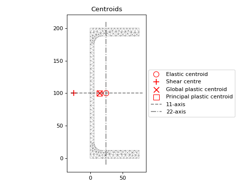
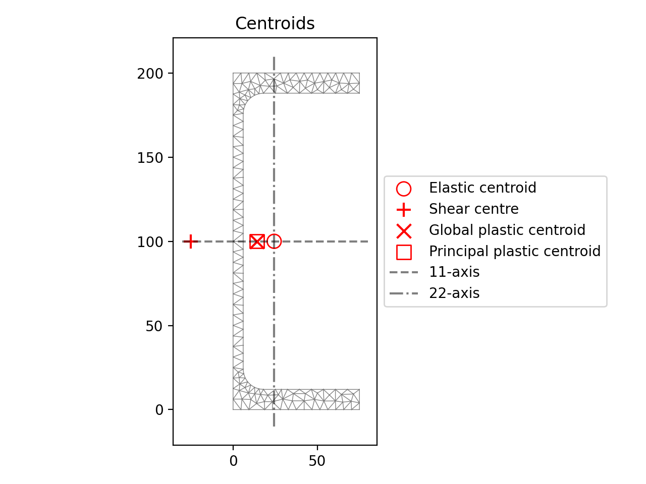
The following example analyses a 200 PFC section and displays a plot of the centroids:

from sectionproperties.pre.library import channel_section
from sectionproperties.analysis import Section

geom = channel_section(d=200, b=75, t_f=12, t_w=6, r=12, n_r=8)
geom.create_mesh(mesh_sizes=[20])

section = Section(geometry=geom)
section.calculate_geometric_properties()
section.calculate_warping_properties()
section.calculate_plastic_properties()

section.plot_centroids()

(Source code, png, hires.png, pdf)

200PFC centroids

Plotting Cross-Section Stresses

After conducting a stress analysis of a cross-section based on applied actions, the resulting stresses can be visualised using any of the plot_stress(), plot_stress_vector() or plot_mohrs_circles() methods.

Plot Stress Contours

StressPost.plot_stress(stress: str, title: str | None = None, cmap: str = 'coolwarm', stress_limits: tuple[float, float] | None = None, normalize: bool = True, fmt: str = '{x:.4e}', colorbar_label: str = 'Stress', alpha: float = 0.5, material_list: list[Material] | None = None, **kwargs: Any) → matplotlib.axes.Axes

Plots filled stress contours over the finite element mesh.

Parameters:

• stress (str) – Type of stress to plot, see below for allowable values

• title (str | None) – Plot title, if None uses default plot title for selected stress

• cmap (str) – Matplotlib color map, see https://matplotlib.org/stable/tutorials/colors/colormaps.html for more detail

• stress_limits (tuple[float, float] | None) – Custom colorbar stress limits (sig_min, sig_max), values outside these limits will appear as white

• normalize (bool) – If set to True, CenteredNorm is used to scale the colormap, if set to False, the default linear scaling is used

• fmt (str) – Number formatting string, see https://docs.python.org/3/library/string.html

• colorbar_label (str) – Colorbar label

• alpha (float) – Transparency of the mesh outlines: \(0 \leq \alpha \leq 1\)

• material_list (list[Material] | None) – If specified, only plots materials present in the list. If set to None, plots all materials.

• kwargs (Any) – Passed to plotting_context()

Raises:

RuntimeError – If the plot failed to be generated

Returns:

Matplotlib axes object

Return type:

matplotlib.axes.Axes

Stress contour plotting options

In general the stresses are described by an action followed by a stress direction (action)_(stress-direction), e.g. mzz_zx represents the shear stress in the zx direction caused by the torsion mzz.

Below is a list of the acceptable values for stress:

• stress="n_zz" - normal stress \(\sigma_{zz,N}\) resulting from the axial load \(N\)

• stress="mxx_zz" - normal stress \(\sigma_{zz,Mxx}\) resulting from the bending moment \(M_{xx}\)

• stress="myy_zz" - normal stress \(\sigma_{zz,Myy}\) resulting from the bending moment \(M_{yy}\)

• stress="m11_zz" - normal stress \(\sigma_{zz,M11}\) resulting from the bending moment \(M_{11}\)

• stress="m22_zz" - normal stress \(\sigma_{zz,M22}\) resulting from the bending moment \(M_{22}\)

• stress="m_zz" - normal stress \(\sigma_{zz,\Sigma M}\) resulting from all bending moments \(M_{xx} + M_{yy} + M_{11} + M_{22}\)

• stress="mzz_zx" - x component of the shear stress \(\sigma_{zx,Mzz}\) resulting from the torsion moment \(M_{zz}\)

• stress="mzz_zy" - y component of the shear stress \(\sigma_{zy,Mzz}\) resulting from the torsion moment \(M_{zz}\)

• stress="mzz_zxy" - resultant shear stress \(\sigma_{zxy,Mzz}\) resulting from the torsion moment \(M_{zz}\)

• stress="vx_zx" - x component of the shear stress \(\sigma_{zx,Vx}\) resulting from the shear force \(V_{x}\)

• stress="vx_zy" - y component of the shear stress \(\sigma_{zy,Vx}\) resulting from the shear force \(V_{x}\)

• stress="vx_zxy" - resultant shear stress \(\sigma_{zxy,Vx}\) resulting from the shear force \(V_{x}\)

• stress="vy_zx" - x component of the shear stress \(\sigma_{zx,Vy}\) resulting from the shear force \(V_{y}\)

• stress="vy_zy" - y component of the shear stress \(\sigma_{zy,Vy}\) resulting from the shear force \(V_{y}\)

• stress="vy_zxy" - resultant shear stress \(\sigma_{zxy,Vy}\) resulting from the shear force \(V_{y}\)

• stress="v_zx" - x component of the shear stress \(\sigma_{zx,\Sigma V}\) resulting from the sum of the applied shear forces \(V_{x} + V_{y}\).

• stress="v_zy" - y component of the shear stress \(\sigma_{zy,\Sigma V}\) resulting from the sum of the applied shear forces \(V_{x} + V_{y}\).

• stress="v_zxy" - resultant shear stress \(\sigma_{zxy,\Sigma V}\) resulting from the sum of the applied shear forces \(V_{x} + V_{y}\)

• stress="zz" - combined normal stress \(\sigma_{zz}\) resulting from all actions

• stress="zx" - x component of the shear stress \(\sigma_{zx}\) resulting from all actions

• stress="zy" - y component of the shear stress \(\sigma_{zy}\) resulting from all actions

• stress="zxy" - resultant shear stress \(\sigma_{zxy}\) resulting from all actions

• stress="11" - major principal stress \(\sigma_{11}\) resulting from all actions

• stress="33" - minor principal stress \(\sigma_{33}\) resulting from all actions

• stress="vm" - von Mises stress \(\sigma_{vM}\) resulting from all actions

Example

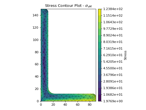
The following example plots a contour of the von Mises stress within a 150 x 90 x 12 UA section resulting from the following actions:

• \(N = 50\) kN

• \(M_{xx} = -5\) kN.m

• \(M_{22} = 2.5\) kN.m

• \(M_{zz} = 1.5\) kN.m

• \(V_x = 10\) kN

• \(V_y = 5\) kN

from sectionproperties.pre.library import angle_section
from sectionproperties.analysis import Section

# create geometry, mesh and section
geom = angle_section(d=150, b=90, t=12, r_r=10, r_t=5, n_r=8)
geom.create_mesh(mesh_sizes=20)
sec = Section(geometry=geom)

# conduct analyses
sec.calculate_geometric_properties()
sec.calculate_warping_properties()
stress = sec.calculate_stress(
    n=50e3, mxx=-5e6, m22=2.5e6, mzz=0.5e6, vx=10e3, vy=5e3
)

# plot stress contour
stress.plot_stress(stress="vm", cmap="viridis", normalize=False)

(Source code, png, hires.png, pdf)

Contour plot of the von Mises stress

Plot Stress Vectors

StressPost.plot_stress_vector(stress: str, title: str | None = None, cmap: str = 'YlOrBr', normalize: bool = False, fmt: str = '{x:.4e}', colorbar_label: str = 'Stress', alpha: float = 0.2, **kwargs: Any) → Axes

Plots stress vectors over the finite element mesh.

Parameters:

• stress (str) – Type of stress to plot, see below for allowable values

• title (str | None) – Plot title, if None uses default plot title for selected stress

• cmap (str) – Matplotlib color map, see https://matplotlib.org/stable/tutorials/colors/colormaps.html for more detail

• normalize (bool) – If set to True, CenteredNorm is used to scale the colormap, if set to False, the default linear scaling is used

• fmt (str) – Number formatting string, see https://docs.python.org/3/library/string.html

• colorbar_label (str) – Colorbar label

• alpha (float) – Transparency of the mesh outlines: \(0 \leq \alpha \leq 1\)

• kwargs (Any) – Passed to plotting_context()

Raises:

RuntimeError – If the plot failed to be generated

Returns:

Matplotlib axes object

Return type:

Axes

Stress vector plotting options

Below is a list of the acceptable values for stress:

• stress="mzz_zxy" - resultant shear stress \(\sigma_{zxy,Mzz}\) resulting from the torsion moment \(M_{zz}\)

• stress="vx_zxy" - resultant shear stress \(\sigma_{zxy,Vx}\) resulting from the shear force \(V_{x}\)

• stress="vy_zxy" - resultant shear stress \(\sigma_{zxy,Vy}\) resulting from the shear force \(V_{y}\)

• stress="v_zxy" - resultant shear stress \(\sigma_{zxy,\Sigma V}\) resulting from the sum of the applied shear forces \(V_{x} + V_{y}\)

• stress="zxy" - resultant shear stress \(\sigma_{zxy}\) resulting from all actions

Example

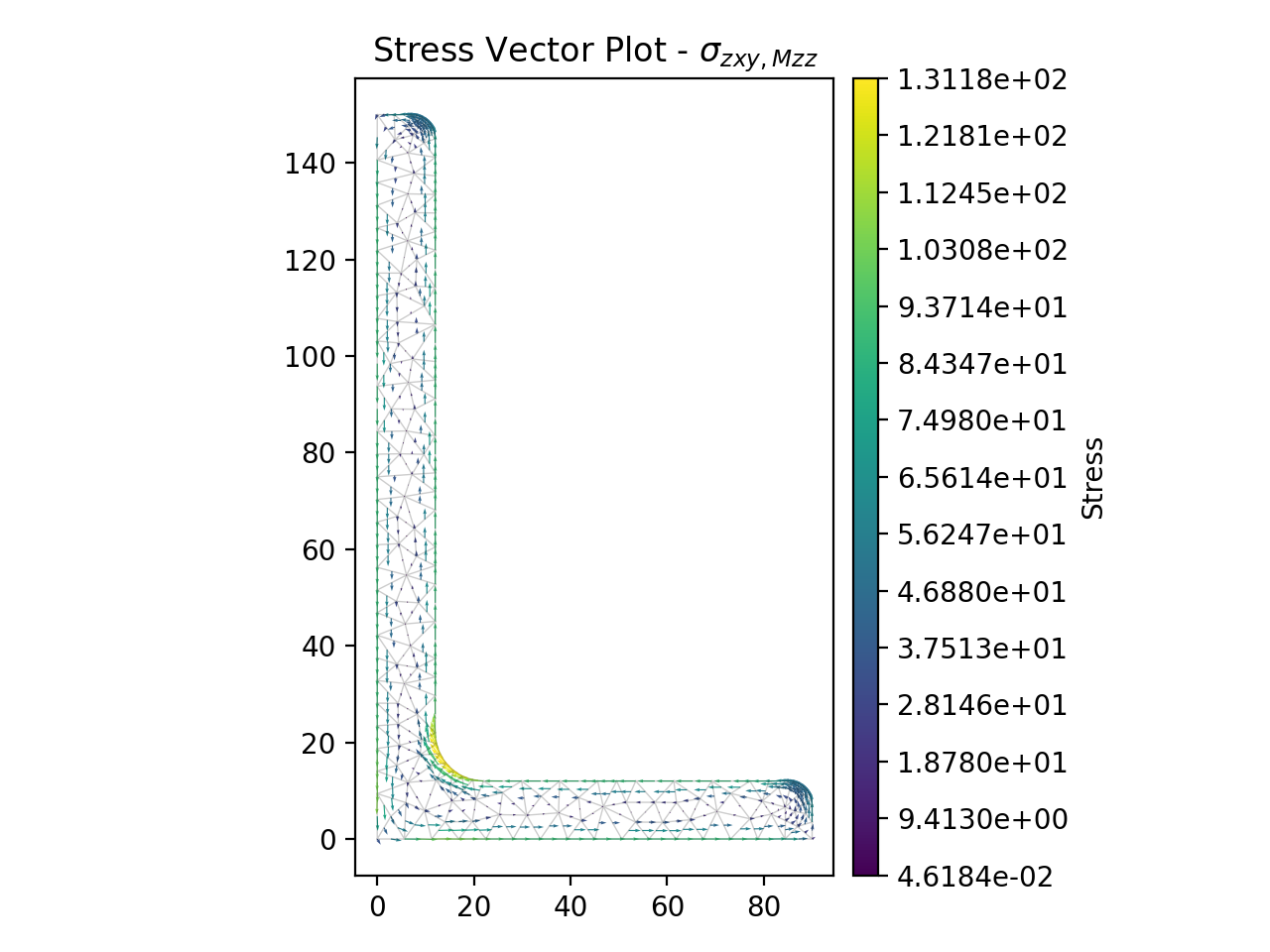
The following example generates a vector plot of the shear stress within a 150 x 90 x 12 UA section resulting from a torsion moment of 1 kN.m:

from sectionproperties.pre.library import angle_section
from sectionproperties.analysis import Section

# create geometry, mesh and section
geom = angle_section(d=150, b=90, t=12, r_r=10, r_t=5, n_r=8)
geom.create_mesh(mesh_sizes=20)
sec = Section(geometry=geom)

# conduct analyses
sec.calculate_geometric_properties()
sec.calculate_warping_properties()
stress = sec.calculate_stress(mzz=1e6)

# plot stress contour
stress.plot_stress_vector(stress="mzz_zxy", cmap="viridis", normalize=False)

(Source code, png, hires.png, pdf)

Contour plot of the von Mises stress

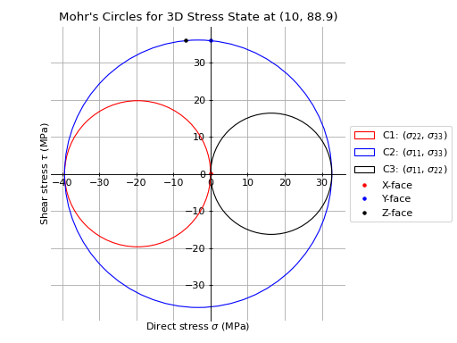
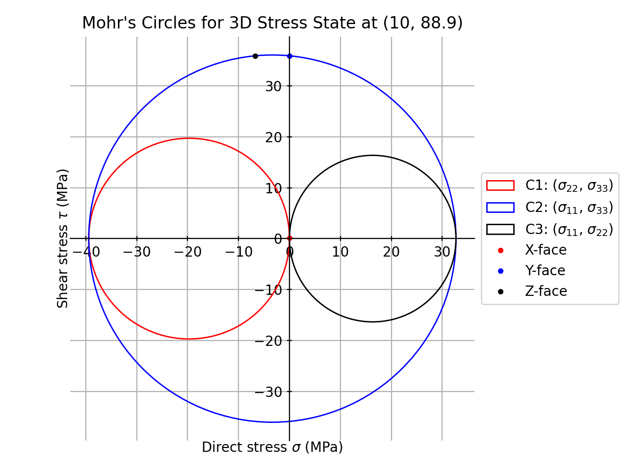
Plot Mohr’s Circles

StressPost.plot_mohrs_circles(x: float, y: float, title: str | None = None, **kwargs: Any) → Axes

Plots Mohr’s circles of the 3D stress state at position (x, y).

Parameters:

• x (float) – x-coordinate of the point to draw Mohr’s Circle

• y (float) – y-coordinate of the point to draw Mohr’s Circle

• title (str | None) – Plot title, if None uses default plot title “Mohr’s Circles for 3D Stress State at {pt}”

• kwargs (Any) – Passed to plotting_context()

Raises:

• ValueError – If the point (x, y) is not within the mesh

• RuntimeError – If the plot failed to be generated

Returns:

Matplotlib axes object

Return type:

Axes

Example

The following example plots the Mohr’s circles for the 3D stress state within a 150x90x12 UA section at the point x=10, y=88.9 resulting from the following actions:

• \(N = 50\) kN

• \(M_{xx} = -5\) kN.m

• \(M_{22} = 2.5\) kN.m

• \(M_{zz} = 1.5\) kN.m

• \(V_{x} = 10\) kN

• \(V_{y} = 5\) kN

from sectionproperties.pre.library import angle_section
from sectionproperties.analysis import Section

# create geometry and section
geom = angle_section(d=150, b=90, t=12, r_r=10, r_t=5, n_r=8)
geom.create_mesh(mesh_sizes=[0])
sec = Section(geometry=geom)

# perform analysis
sec.calculate_geometric_properties()
sec.calculate_warping_properties()
post = sec.calculate_stress(
    n=50e3, mxx=-5e6, m22=2.5e6, mzz=0.5e6, vx=10e3, vy=5e3
)

# plot mohr's circle
post.plot_mohrs_circles(x=10, y=88.9)

(Source code, png, hires.png, pdf)

Mohr’s circles for a 150x90x12 UA

Retrieving Cross-Section Stresses

Numerical values for cross-section stress can also be obtained with the get_stress_at_points() and get_stress() methods.

Get Stress at Points

This method can be used to obtain the stress at one or multiple points. A geometric analysis must be performed prior to calling this method. Further, if the shear force or torsion is non-zero, a warping analysis must also be performed. See Retrieving Stresses for an example of how this method can be used to plot the stress distribution along a line.

Section.get_stress_at_points(pts: list[tuple[float, float]], n: float = 0.0, mxx: float = 0.0, myy: float = 0.0, m11: float = 0.0, m22: float = 0.0, mzz: float = 0.0, vx: float = 0.0, vy: float = 0.0, agg_func: ~typing.Callable[[list[float]], float] = <function average>) → list[tuple[float, float, float] | None]

Calculates the stress for a list of points.

Calculates the stress at a set of points within an element for given design actions and returns the global stress components for each point.

Parameters:

• pts (list[tuple[float, float]]) – A list of points [(x, y), ..., ]

• n (float) – Axial force

• mxx (float) – Bending moment about the centroidal xx-axis

• myy (float) – Bending moment about the centroidal yy-axis

• m11 (float) – Bending moment about the centroidal 11-axis

• m22 (float) – Bending moment about the centroidal 22-axis

• mzz (float) – Torsion moment about the centroidal zz-axis

• vx (float) – Shear force acting in the x-direction

• vy (float) – Shear force acting in the y-direction

• agg_func (Callable[[list[float]], float]) – A function that aggregates the stresses if the point is shared by several elements. If the point, pt, is shared by several elements (e.g. if it is a node or on an edge), the stresses are retrieved from each element and combined according to this function.

Raises:

RuntimeError – If a warping analysis has not been carried out and a shear force or a torsion moment is supplied

Returns:

Resultant normal and shear stresses (sigma_zz, tau_xz, tau_yz) for each point pt. If a point is not in the section then None is returned for that element in the list.

Return type:

list[tuple[float, float, float] | None]

General Get Stress

This method must be used after a stress analysis. It returns a data structure containing all the stresses within the cross-section, grouped by material.

StressPost.get_stress() → list[dict[str, object]]

Returns the stresses within each material.

Returns:

A list of dictionaries containing the cross-section stresses at each node for each material

Return type:

list[dict[str, object]]

Note

Each list of stresses in the dictionary contains the stresses at every node (order from node 0 to node n) in the entire mesh. As a result, when the current material does not exist at a node, a value of zero will be reported.

Dictionary keys and values

In general the stresses are described by an action followed by a stress direction (action)_(stress-direction), e.g. mzz_zx represents the shear stress in the zx direction caused by the torsion mzz.

Below is a list of the returned dictionary keys and values:

• "material" - material name

• "sig_zz_n" - normal stress \(\sigma_{zz,N}\) resulting from the axial load \(N\)

• "sig_zz_mxx" - normal stress \(\sigma_{zz,Mxx}\) resulting from the bending moment \(M_{xx}\)

• "sig_zz_myy" - normal stress \(\sigma_{zz,Myy}\) resulting from the bending moment \(M_{yy}\)

• "sig_zz_m11" - normal stress \(\sigma_{zz,M11}\) resulting from the bending moment \(M_{11}\)

• "sig_zz_m22" - normal stress \(\sigma_{zz,M22}\) resulting from the bending moment \(M_{22}\)

• "sig_zz_m" - normal stress \(\sigma_{zz,\Sigma M}\) resulting from all bending moments \(M_{xx} + M_{yy} + M_{11} + M_{22}\)

• "sig_zx_mzz" - x component of the shear stress \(\sigma_{zx,Mzz}\) resulting from the torsion moment \(M_{zz}\)

• "sig_zy_mzz" - y component of the shear stress \(\sigma_{zy,Mzz}\) resulting from the torsion moment \(M_{zz}\)

• "sig_zxy_mzz" - resultant shear stress \(\sigma_{zxy,Mzz}\) resulting from the torsion moment \(M_{zz}\)

• "sig_zx_vx" - x component of the shear stress \(\sigma_{zx,Vx}\) resulting from the shear force \(V_{x}\)

• "sig_zy_vx" - y component of the shear stress \(\sigma_{zy,Vx}\) resulting from the shear force \(V_{x}\)

• "sig_zxy_vx" - resultant shear stress \(\sigma_{zxy,Vx}\) resulting from the shear force \(V_{x}\)

• "sig_zx_vy" - x component of the shear stress \(\sigma_{zx,Vy}\) resulting from the shear force \(V_{y}\)

• "sig_zy_vy" - y component of the shear stress \(\sigma_{zy,Vy}\) resulting from the shear force \(V_{y}\)

• "sig_zxy_vy" - resultant shear stress \(\sigma_{zxy,Vy}\) resulting from the shear force \(V_{y}\)

• "sig_zx_v" - x component of the shear stress \(\sigma_{zx,\Sigma V}\) resulting from the sum of the applied shear forces \(V_{x} + V_{y}\).

• "sig_zy_v" - y component of the shear stress \(\sigma_{zy,\Sigma V}\) resulting from the sum of the applied shear forces \(V_{x} + V_{y}\).

• "sig_zxy_v" - resultant shear stress \(\sigma_{zxy,\Sigma V}\) resulting from the sum of the applied shear forces \(V_{x} + V_{y}\)

• "sig_zz" - combined normal stress \(\sigma_{zz}\) resulting from all actions

• "sig_zx" - x component of the shear stress \(\sigma_{zx}\) resulting from all actions

• "sig_zy" - y component of the shear stress \(\sigma_{zy}\) resulting from all actions

• "sig_zxy" - resultant shear stress \(\sigma_{zxy}\) resulting from all actions

• "sig_11" - major principal stress \(\sigma_{11}\) resulting from all actions

• "sig_33" - minor principal stress \(\sigma_{33}\) resulting from all actions

• "sig_vm" - von Mises stress \(\sigma_{vM}\) resulting from all actions