Overview#

The process of performing a cross-section analysis with sectionproperties can be broken down into three stages:

Pre-Processor: The input geometry, materials and finite element mesh is created.
Solver: The cross-section properties are determined.
Post-Processor: The results are presented in a number of different formats.

Pre-Processor#

The shape of the cross-section and corresponding materials define the geometry of the cross-section. There are many different ways to create geometry in sectionproperties, more information can be found in Geometry.

The final stage in the pre-processor involves generating a finite element mesh of the geometry that the solver can use to calculate the cross-section properties. This can easily be performed using the create_mesh() method that all Geometry objects have access to.

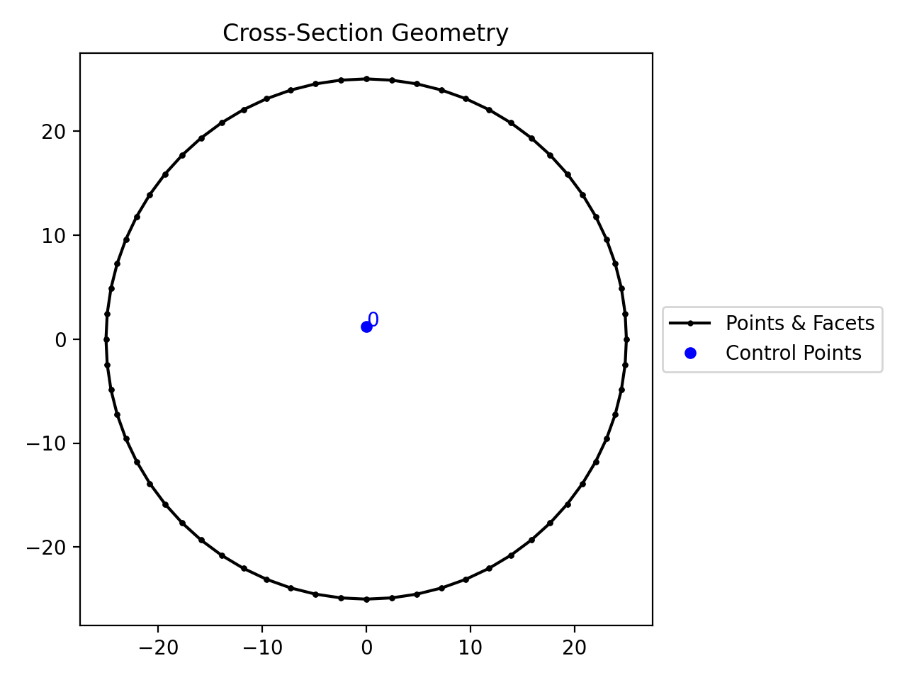
The following example creates a geometry object with a circular cross-section. The diameter of the circle is 50 mm and 64 points are used to discretise the circumference of the circle. A finite element mesh is generated with a maximum triangular area of 2.5 mm² and the geometry is plotted.

from sectionproperties.pre.library import circular_section

geom = circular_section(d=50, n=64)
geom.create_mesh(mesh_sizes=[2.5])
geom.plot_geometry()

(Source code, png, hires.png, pdf)

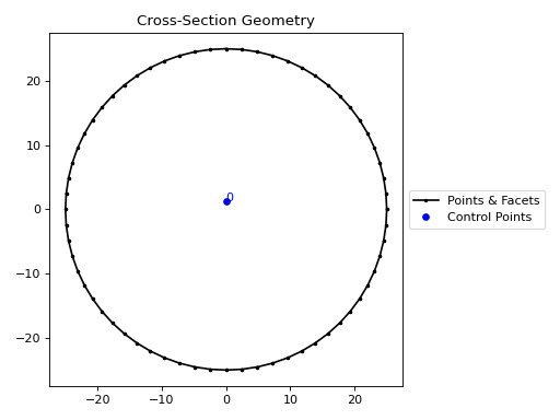
../_images/overview-1.png — Circular Section#

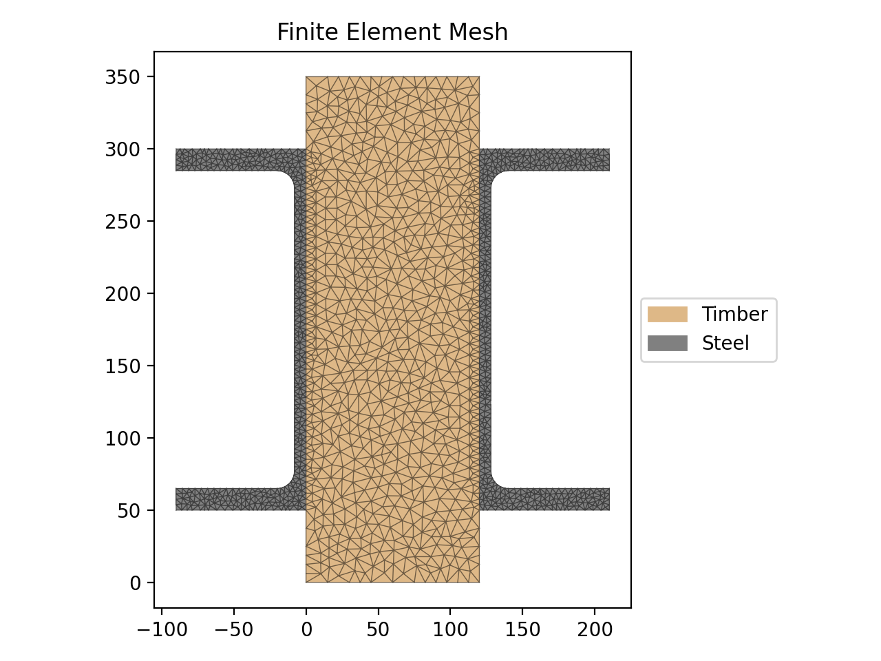
If you are analysing a composite section, or would like to include material properties in your model, material properties can be created using the Material class. The following example creates a steel-timber composite section and plots the mesh.

from sectionproperties.pre import Material
from sectionproperties.pre.library import rectangular_section, channel_section
from sectionproperties.analysis import Section

# create materials
steel = Material(
    name="Steel",
    elastic_modulus=200e3,
    poissons_ratio=0.3,
    density=7.85e-6,
    yield_strength=500,
    color="grey",
)
timber = Material(
    name="Timber",
    elastic_modulus=8e3,
    poissons_ratio=0.35,
    density=6.5e-7,
    yield_strength=20,
    color="burlywood",
)

# create individual geometry objects
pfc = channel_section(d=250, b=90, t_f=15, t_w=8, r=12, n_r=8, material=steel)
rect = rectangular_section(d=350, b=120, material=timber)
pfc_right = pfc.align_center(align_to=rect).align_to(other=rect, on="right")
pfc_left = pfc_right.mirror_section(axis="y", mirror_point=(60, 0))

# combine into single geometry and mesh
geom = rect + pfc_left + pfc_right
geom.create_mesh(mesh_sizes=[50.0, 10.0, 10.0])

# create section object and plot the mesh
sec = Section(geometry=geom)
sec.plot_mesh()

(Source code, png, hires.png, pdf)

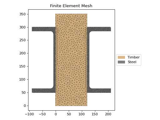
../_images/overview-2.png — Steel-Timber Composite Section#

Solver#

The solver operates on a Section object and can perform five different analysis types:

Geometric Analysis: calculates area properties, calculate_geometric_properties().
Warping Analysis: calculates torsion and shear properties, calculate_warping_properties().
Frame Analysis: calculates section properties used for frame analysis (more efficient than running a geometric and warping analysis), calculate_frame_properties().
Plastic Analysis: calculates plastic properties, calculate_plastic_properties().
Stress Analysis: calculates cross-section stresses, calculate_stress().

Post-Processor#

There are a number of built-in methods to enable the post-processing of analysis results. For example, a full list of calculated section properties can be printed to the terminal by using the display_results() method. Alternatively, specific properties can be retrieved by calling the appropriate get method, e.g. get_ic().

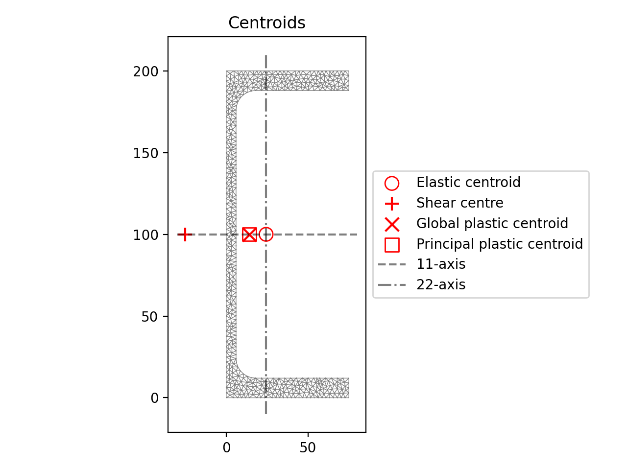
The calculated cross-section centroids can be plotted by calling the plot_centroids() method. The following example plots the centroids of a 200 PFC section:

from sectionproperties.pre.library import channel_section
from sectionproperties.analysis import Section

geom = channel_section(d=200, b=75, t_f=12, t_w=6, r=12, n_r=8)
geom.create_mesh(mesh_sizes=[5.0])

sec = Section(geom)
sec.calculate_geometric_properties()
sec.calculate_plastic_properties()
sec.calculate_warping_properties()

sec.plot_centroids()

(Source code, png, hires.png, pdf)

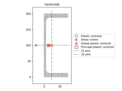
../_images/overview-3.png — 200 PFC elastic, plastic and shear centroids#

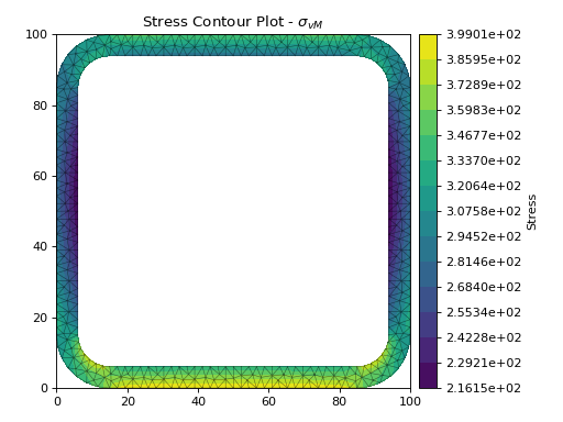
Finally, cross-section stresses may be retrieved by at specific points by calling the get_stress_at_points() method, or plotted by calling the plot_stress() method from a StressPost object, obtained after running the calculate_stress() method. The following example plots the von Mises stress in a 100 x 6 SHS subject to bending, shear and torsion:

from sectionproperties.pre.library import rectangular_hollow_section
from sectionproperties.analysis import Section

geom = rectangular_hollow_section(d=100, b=100, t=6, r_out=15, n_r=8)
geom.create_mesh(mesh_sizes=[5.0])

sec = Section(geom)
sec.calculate_geometric_properties()
sec.calculate_warping_properties()
stress = sec.calculate_stress(vx=20e3, mxx=15e6, mzz=15e6)

stress.plot_stress(stress="vm", cmap="viridis", normalize=False)

(Source code, png, hires.png, pdf)

../_images/overview-4.png — 100 x 6 SHS von Mises stress#