Pilkey - Composite Rectangular Strip

This example re-creates the numerical example “B.8 Composite Rectangular Strip” on page 454 of “Analysis and Design of Elastic Beams” by Walter D. Pilkey. Note that this example is the same as Example 5.13.

BibTeX reference:

@book{Pilkey,
    author = {Pilkey, Walter D},
    booktitle = {Analysis and Design of Elastic Beams},
    edition = {First},
    isbn = {0471381527},
    language = {eng},
    publisher = {Wiley},
    title = {Analysis and Design of Elastic Beams: Computational Methods},
    year = {2002},
}

Problem Description

A non-homogenous rectangular cross-section of 30 in. x 2 in. is analysed, see the figure below. The left hand side consists of Aluminium, while the right consists of Copper. The material properties are summarised below:

Aluminium

• E = 10400000

• nu = 0.3

Copper

• E = 18500000

• nu = 0.3

Note that sectionproperties uses an x-y coordinate system rather than the y-z system used by Pilkey.

from IPython.display import Image


display(Image(filename="images/comp-geom.png"))

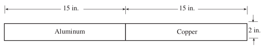
We can model the above geometry by creating two rectangles and aligning the right-hand rectangle to the right-side of that on the left.

from sectionproperties.pre import Material
from sectionproperties.pre.library import rectangular_section


d = 2  # depth of rectangles
b = 15  # width of each rectangle
# aluminium material
al = Material(
    name="Aluminium",
    elastic_modulus=10.4e6,
    poissons_ratio=0.3,
    yield_strength=1.0,
    density=1.0,
    color="lightgrey",
)
# aluminium material
cu = Material(
    name="Copper",
    elastic_modulus=18.5e6,
    poissons_ratio=0.3,
    yield_strength=1.0,
    density=1.0,
    color="gold",
)

# create two rectangles and add geometry together
geom_al = rectangular_section(d=d, b=b, material=al)
geom_cu = rectangular_section(d=d, b=b, material=cu).align_to(other=geom_al, on="right")
geom = geom_al + geom_cu

# plot geometry
geom.plot_geometry()

<Axes: title={'center': 'Cross-Section Geometry'}>

Create mesh and Section object

The numerical analysis by Pilkey uses 9-noded quadraliteral elements. The mesh used by Pilkey for this problem can be seen below.

display(Image(filename="images/comp-mesh.png"))

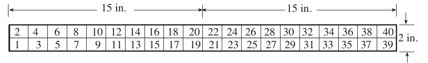
We can create a mesh in sectionproperties using 6-noded triangular elements by defining a maximum triangular element area. In this case we choose mesh_sizes=0.1 and create the resulting Section object.

from sectionproperties.analysis import Section


geom.create_mesh(mesh_sizes=0.1)
sec = Section(geometry=geom)
sec.plot_mesh()

<Axes: title={'center': 'Finite Element Mesh'}>

Calculate Cross-Section Properties

Pilkey reports both geometric and warping properties, as such we conduct both analyses.

sec.calculate_geometric_properties()
sec.calculate_warping_properties()

Comparison of Results

The numerical results obtained by Pilkey is listed in the dictionary below.

pilkey = {
    "area": 60,
    "ea_ref": 83.36,
    "j_ref": 106.22,
}

Pilkey uses aluminium as the reference material, so we will do the same.

sectionproperties = {
    "area": sec.get_area(),
    "ea_ref": sec.get_ea(e_ref=al),
    "j_ref": sec.get_ej(e_ref=al),
}

The comparison of results is summarised in the table below. Relative error is reported in all cases.

from rich.console import Console
from rich.table import Table
from rich.text import Text


# setup table
table = Table(title="Comparison of Results")
table.add_column("Property", justify="left", style="cyan", no_wrap=True)
table.add_column(Text("Pilkey", justify="center"), justify="right", style="green")
table.add_column(Text("sectionproperties", style="i"), justify="right", style="green")
table.add_column(Text("Error", justify="center"), justify="right", style="green")

# create a row for each property
for key in pilkey:
    # get results
    p_res = pilkey[key]
    sp_res = sectionproperties[key]

    # calculate relative error
    if p_res != 0:
        rel_error = (sp_res - p_res) / p_res
    else:
        rel_error = sp_res

    # print row
    table.add_row(key, f"{p_res:.4e}", f"{sp_res:.4e}", f"{rel_error:.2e}")

console = Console()
console.print(table)

                  Comparison of Results                  
┏━━━━━━━━━━┳━━━━━━━━━━━━┳━━━━━━━━━━━━━━━━━━━┳━━━━━━━━━━━┓
┃ Property ┃   Pilkey   ┃ sectionproperties ┃   Error   ┃
┡━━━━━━━━━━╇━━━━━━━━━━━━╇━━━━━━━━━━━━━━━━━━━╇━━━━━━━━━━━┩
│ area     │ 6.0000e+01 │        6.0000e+01 │ -8.29e-16 │
│ ea_ref   │ 8.3360e+01 │        8.3365e+01 │  6.46e-05 │
│ j_ref    │ 1.0622e+02 │        1.0612e+02 │ -9.30e-04 │
└──────────┴────────────┴───────────────────┴───────────┘

Pilkey notes that the analytical formula for such a geometry has been derived by Muskhelishvili (1953):

\[J = \frac{1}{3} (L_a + \mu L_c) t^3 - 3.361 \frac{t^4}{16} \frac{1 + {\mu}^2}{1 + \mu}\]

where:

\[\mu = \frac{G_c}{G_a} = \frac{E_c}{E_a} = \frac{18.5}{10.4}\]

This expression evaluates to \(J=106.12\) in\(^4\), which aligns closer to the result from sectionproperties than that obtained by Pilkey.

mu = 18.5 / 10.4
j_an = 1 / 3 * (b + mu * b) * d**3 - 3.361 * (d**4) / (16) * (1 + mu**2) / (1 + mu)
print(f"J_an = {j_an:.4f} mm4")
print(f"J_sp = {sectionproperties['j_ref']:.4f} mm4")
print(f"J_pi = {pilkey['j_ref']:.4f} mm4")

J_an = 106.1172 mm4
J_sp = 106.1212 mm4
J_pi = 106.2200 mm4