Pilkey - Circular Arc

This example re-creates the numerical example “B.7 Circular Arc” on page 451 of “Analysis and Design of Elastic Beams” by Walter D. Pilkey.

BibTeX reference:

@book{Pilkey,
    author = {Pilkey, Walter D},
    booktitle = {Analysis and Design of Elastic Beams},
    edition = {First},
    isbn = {0471381527},
    language = {eng},
    publisher = {Wiley},
    title = {Analysis and Design of Elastic Beams: Computational Methods},
    year = {2002},
}

Problem Description

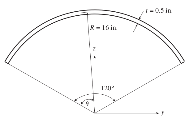
A circular arc of 120\(^{\circ}\) and radius of 16 in. is analysed, see the figure below. The material properties of the section are taken to be E=210000000 and nu=0.33333. Note that the elastic modulus plays no role in this analysis as the geometry is homogenous, however its value is included for completeness. Also note that the value for E used by Pilkey is in kPa (steel), whereas the problem is defined in inches - this mixing of units is not an issue due to the elastic modulus not affecting the geometric results.

Note that sectionproperties uses an x-y coordinate system rather than the y-z system used by Pilkey.

from IPython.display import Image


display(Image(filename="images/arc-geom.png"))

We can model the above geometry by generating a shapely LineString from a list of points defining the centreline of the above arc. The LineString can be buffered (extruded) orthogonal to the line to create a Polygon object. This Polygon object can then be passed to the sectionproperties Geometry object.

import numpy as np
from shapely import LineString, Polygon, buffer

from sectionproperties.pre import Geometry, Material


r = 16  # radius
t = 0.5  # thickness
alpha = 2 * np.pi / 3  # arc angle
n = 128  # number of points definining LineString
# steel material
mat = Material(
    name="Steel",
    elastic_modulus=2.1e8,
    poissons_ratio=0.33333,
    yield_strength=1.0,
    density=1.0,
    color="lightgrey",
)

# define points on the LineString
pts = []
for idx in range(n):
    theta = -alpha / 2 + idx / (n - 1) * alpha
    x = r * np.sin(theta)
    y = r * np.cos(theta)
    pts.append((x, y))

# create LineString
line = LineString(coordinates=pts)

# create Polygon by buffering the LineString
poly = buffer(geometry=line, distance=0.5 * t, cap_style="flat", join_style="mitre")

# create sectionproperties Geometry object
geom = Geometry(geom=poly, material=mat)

# plot geometry
geom.plot_geometry()

<Axes: title={'center': 'Cross-Section Geometry'}>

Create mesh and Section object

The numerical analysis by Pilkey uses 9-noded quadraliteral elements. The mesh used by Pilkey for this problem can be seen below.

display(Image(filename="images/arc-mesh.png"))

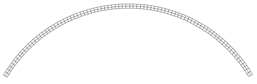
We can create a mesh in sectionproperties using 6-noded triangular elements by defining a maximum triangular element area. In this case we choose mesh_sizes=0.1 and create the resulting Section object.

from sectionproperties.analysis import Section


geom.create_mesh(mesh_sizes=0.1)
sec = Section(geometry=geom)
sec.plot_mesh()

<Axes: title={'center': 'Finite Element Mesh'}>

Calculate Cross-Section Properties

Pilkey reports both geometric and warping properties, as such we conduct both analyses.

sec.calculate_geometric_properties()
sec.calculate_warping_properties()

Comparison of Results

The numerical results obtained by Pilkey is listed in the dictionary below.

pilkey = {
    "area": 16.75516,
    "qx": 221.72054,
    "qy": 0.0,
    "cx": 0.0,
    "cy": 13.23297,
    "x_sc": 0.0,
    "y_sc": 17.83662,
    "ixx_g": 3032.21070,
    "iyy_g": 1258.15764,
    "ixy_g": 0.0,
    "ixx_c": 98.18931,
    "iyy_c": 1258.15764,
    "ixy_c": 0.0,
    "zxx": 18.32584,
    "zyy": 89.40279,
    "rx": 2.42079,
    "ry": 8.66549,
    "phi": -90.0,
    "alpha_x": 1.50823,
    "alpha_y": 4.60034,
    "alpha_xy": 0.0,
    "j": 1.38355,
    "gamma": 1046.49221,
}

Most of these results can be directly obtained from sectionproperties, the only properties that require calculation are the shear coefficients, alpha. The shear coefficient can be obtained from the shear area as follows:

\(\alpha = \frac{A}{A_s}\)

where \(A\) is the cross-section area and \(A_s\) is the shear area.

We create a similar dictionary for the sectionproperties results.

sectionproperties = {
    "area": sec.get_area(),
    "qx": sec.get_eq(e_ref=mat)[0],
    "qy": sec.get_eq(e_ref=mat)[1],
    "cx": sec.get_c()[0],
    "cy": sec.get_c()[1],
    "x_sc": sec.get_sc()[0],
    "y_sc": sec.get_sc()[1],
    "ixx_g": sec.get_eig(e_ref=mat)[0],
    "iyy_g": sec.get_eig(e_ref=mat)[1],
    "ixy_g": sec.get_eig(e_ref=mat)[2],
    "ixx_c": sec.get_eic(e_ref=mat)[0],
    "iyy_c": sec.get_eic(e_ref=mat)[1],
    "ixy_c": sec.get_eic(e_ref=mat)[2],
    "zxx": min(sec.get_ez(e_ref=mat)[:2]),
    "zyy": min(sec.get_ez(e_ref=mat)[2:]),
    "rx": sec.get_rc()[0],
    "ry": sec.get_rc()[1],
    "phi": sec.get_phi(),
    "alpha_x": sec.get_area() / sec.get_eas(e_ref=mat)[0],
    "alpha_y": sec.get_area() / sec.get_eas(e_ref=mat)[1],
    "alpha_xy": sec.get_area() / sec.section_props.a_sxy,
    "j": sec.get_ej(e_ref=mat),
    "gamma": sec.get_egamma(e_ref=mat),
}

The comparison of results is summarised in the table below. Relative error is reported in all cases, except where a value is zero, in which the absolute error is reported.

from rich.console import Console
from rich.table import Table
from rich.text import Text


# setup table
table = Table(title="Comparison of Results")
table.add_column("Property", justify="left", style="cyan", no_wrap=True)
table.add_column(Text("Pilkey", justify="center"), justify="right", style="green")
table.add_column(Text("sectionproperties", style="i"), justify="right", style="green")
table.add_column(Text("Error", justify="center"), justify="right", style="green")

# create a row for each property
for key in pilkey:
    # get results
    p_res = pilkey[key]
    sp_res = sectionproperties[key]

    # calculate relative error
    if p_res != 0:
        rel_error = (sp_res - p_res) / p_res
    else:
        rel_error = sp_res

    # print row
    table.add_row(key, f"{p_res:.4e}", f"{sp_res:.4e}", f"{rel_error:.2e}")

console = Console()
console.print(table)

                  Comparison of Results                   
┏━━━━━━━━━━┳━━━━━━━━━━━━━┳━━━━━━━━━━━━━━━━━━━┳━━━━━━━━━━━┓
┃ Property ┃   Pilkey    ┃ sectionproperties ┃   Error   ┃
┡━━━━━━━━━━╇━━━━━━━━━━━━━╇━━━━━━━━━━━━━━━━━━━╇━━━━━━━━━━━┩
│ area     │  1.6755e+01 │        1.6755e+01 │ -1.13e-05 │
│ qx       │  2.2172e+02 │        2.2171e+02 │ -3.44e-05 │
│ qy       │  0.0000e+00 │        1.0424e-12 │  1.04e-12 │
│ cx       │  0.0000e+00 │        6.2217e-14 │  6.22e-14 │
│ cy       │  1.3233e+01 │        1.3233e+01 │ -2.30e-05 │
│ x_sc     │  0.0000e+00 │        1.8959e-13 │  1.90e-13 │
│ y_sc     │  1.7837e+01 │        1.7836e+01 │ -2.11e-05 │
│ ixx_g    │  3.0322e+03 │        3.0320e+03 │ -5.71e-05 │
│ iyy_g    │  1.2582e+03 │        1.2581e+03 │ -5.99e-05 │
│ ixy_g    │  0.0000e+00 │        1.4695e-11 │  1.47e-11 │
│ ixx_c    │  9.8189e+01 │        9.8185e+01 │ -4.73e-05 │
│ iyy_c    │  1.2582e+03 │        1.2581e+03 │ -5.99e-05 │
│ ixy_c    │  0.0000e+00 │        9.0024e-13 │  9.00e-13 │
│ zxx      │  1.8326e+01 │        1.8320e+01 │ -3.23e-04 │
│ zyy      │  8.9403e+01 │        8.9404e+01 │  1.39e-05 │
│ rx       │  2.4208e+00 │        2.4208e+00 │ -1.64e-05 │
│ ry       │  8.6655e+00 │        8.6653e+00 │ -2.40e-05 │
│ phi      │ -9.0000e+01 │       -9.0000e+01 │ -3.16e-16 │
│ alpha_x  │  1.5082e+00 │        1.5082e+00 │  1.92e-06 │
│ alpha_y  │  4.6003e+00 │        4.6003e+00 │ -1.25e-05 │
│ alpha_xy │  0.0000e+00 │        9.4762e-21 │  9.48e-21 │
│ j        │  1.3836e+00 │        1.3836e+00 │  5.87e-05 │
│ gamma    │  1.0465e+03 │        1.0465e+03 │ -3.18e-05 │
└──────────┴─────────────┴───────────────────┴───────────┘

All results are within acceptable limits. Out of the warping properties, the torsion constant had the largest relative error, however this value is relatively small and acceptable given the differences in element type and mesh.

err = (sectionproperties["j"] - pilkey["j"]) / pilkey["j"]
print(f"Torsion Constant Relative Error: {err:.6f}")

Torsion Constant Relative Error: 0.000059