Class for defining the geometry of a contiguous section of a single material.
Provides an interface for the user to specify the geometry defining a section. A method
is provided for generating a triangular mesh, transforming the section (e.g. translation,
rotation, perimeter offset, mirroring), aligning the geometry to another geometry, and
designating stress recovery points.
Variables
geom (shapely.geometry.Polygon) – a Polygon object that defines the geometry
material (Optional[Material]) – Optional, a Material to associate with this geometry
control_point – Optional, an (x, y) coordinate within the geometry that
represents a pre-assigned control point (aka, a region identification point)
to be used instead of the automatically assigned control point generated
with shapely.geometry.Polygon.representative_point().
tol – Optional, default is 12. Number of decimal places to round the geometry vertices
to. A lower value may reduce accuracy of geometry but increases precision when aligning
geometries to each other.
Returns a new Geometry object, translated in both x and y, so that the
the new object’s centroid will be aligned with the centroid of the object
in ‘align_to’. If ‘align_to’ is an x, y coordinate, then the centroid will
be aligned to the coordinate. If ‘align_to’ is None then the new
object will be aligned with its centroid at the origin.
Parameters
align_to (Optional[Union[Geometry, Tuple[float, float]]]) – Another Geometry to align to or None (default is None)
Returns a new Geometry object, representing ‘self’ translated so that is aligned
‘on’ one of the outer bounding box edges of ‘other’.
If ‘other’ is a tuple representing an (x,y) coordinate, then the new
Geometry object will represent ‘self’ translated so that it is aligned
‘on’ that side of the point.
Parameters
other (Union[Geometry, Tuple[float, float]]) – Either another Geometry or a tuple representing an
(x,y) coordinate point that ‘self’ should align to.
on – A str of either “left”, “right”, “bottom”, or “top” indicating which
side of ‘other’ that self should be aligned to.
inner (bool) – Default False. If True, align ‘self’ to ‘other’ in such a way that
‘self’ is aligned to the “inside” of ‘other’. In other words, align ‘self’ to
‘other’ on the specified edge so they overlap.
Returns a new Geometry object with ‘control_point’ assigned as the control point for the
new Geometry. The assignment of a control point is intended to replace the control point
automatically generated by shapely.geometry.Polygon.representative_point().
An assigned control point is carried through and transformed with the Geometry whenever
it is shifted, aligned, mirrored, unioned, and/or rotated. If a perimeter_offset operation is applied,
a check is performed to see if the assigned control point is still valid (within the new region)
and, if so, it is kept. If not, a new control point is auto-generated.
The same check is performed when the geometry undergoes a difference operation (with the ‘-’
operator) or a shift_points operation. If the assigned control point is valid, it is kept. If not,
a new one is auto-generated.
For all other operations (e.g. symmetric difference, intersection, split, ), the assigned control point
is discarded and a new one auto-generated.
Variables
control_points – An (x, y) coordinate that describes the distinct, contiguous,
region of a single material within the geometry.
Exactly one point is required for each geometry with a distinct material.
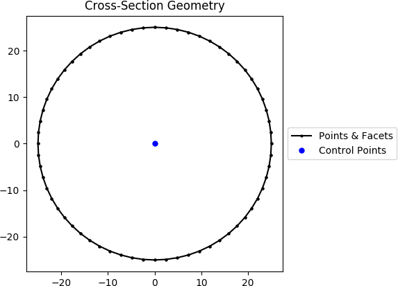
The following example creates a circular cross-section with a diameter of 50 with 64
points, and generates a mesh with a maximum triangular area of 2.5:
Class method to create a Geometry from the objects in a Rhino .3dm file.
Parameters
filepath (Union[str, pathlib.Path]) – File path to the rhino .3dm file.
kwargs – See below.
Raises
RuntimeError – A RuntimeError is raised if two or more polygons are found.
This is dependent on the keyword arguments.
Try adjusting the keyword arguments if this error is raised.
Bézier curve interpolation number. In Rhino a surface’s edges are nurb based curves.
Shapely does not support nurbs, so the individual Bézier curves are interpolated using straight lines.
This parameter sets the number of straight lines used in the interpolation.
Default is 1.
vec1 (numpy.ndarray,optional) –
A 3d vector in the Shapely plane. Rhino is a 3D geometry environment.
Shapely is a 2D geometric library.
Thus a 2D plane needs to be defined in Rhino that represents the Shapely coordinate system.
vec1 represents the 1st vector of this plane. It will be used as Shapely’s x direction.
Default is [1,0,0].
vec2 (numpy.ndarray,optional) –
Continuing from vec1, vec2 is another vector to define the Shapely plane.
It must not be [0,0,0] and it’s only requirement is that it is any vector in the Shapely plane (but not equal to vec1).
Default is [0,1,0].
plane_distance (float,optional) –
The distance to the Shapely plane.
Default is 0.
project (boolean,optional) –
Controls if the breps are projected onto the plane in the direction of the Shapley plane’s normal.
Default is True.
parallel (boolean,optional) –
Controls if only the rhino surfaces that have the same normal as the Shapely plane are yielded.
If true, all non parallel surfaces are filtered out.
Default is False.
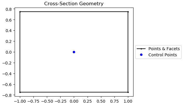
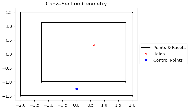
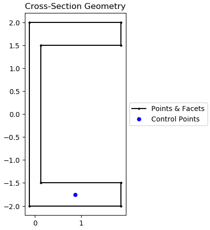
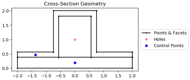
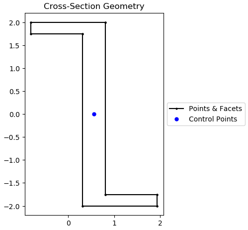
An interface for the creation of Geometry objects through the definition of points,
facets, and holes.
Variables
points (list[list[float, float]]) – List of points (x, y) defining the vertices of the section geometry.
If facets are not provided, it is a assumed the that the list of points are ordered
around the perimeter, either clockwise or anti-clockwise.
facets (list[list[int, int]]) – A list of (start, end) indexes of vertices defining the edges
of the section geoemtry. Can be used to define both external and internal perimeters of holes.
Facets are assumed to be described in the order of exterior perimeter, interior perimeter 1,
interior perimeter 2, etc.
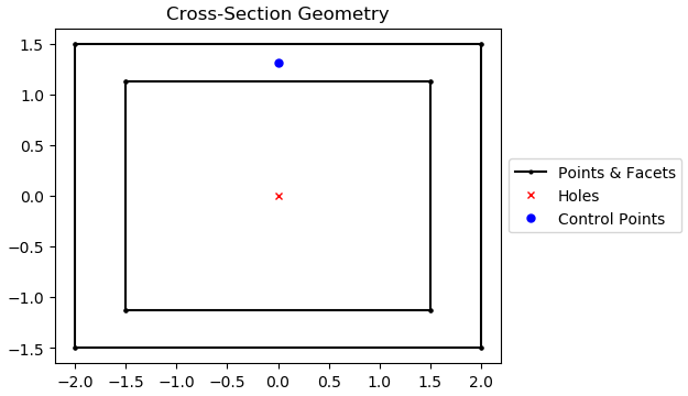
control_points – An (x, y) coordinate that describes the distinct, contiguous,
region of a single material within the geometry. Must be entered as a list of coordinates,
e.g. [[0.5, 3.2]]
Exactly one point is required for each geometry with a distinct material.
If there are multiple distinct regions, then use CompoundGeometry.from_points()
holes (list[list[float, float]]) – Optional. A list of points (x, y) that define interior regions as
being holes or voids. The point can be located anywhere within the hole region.
Only one point is required per hole region.
material – Optional. A Material object
that is to be assigned. If not given, then the
DEFAULT_MATERIAL will be used.
Bézier curve interpolation number. In Rhino a surface’s edges are nurb based curves.
Shapely does not support nurbs, so the individual Bézier curves are interpolated using straight lines.
This parameter sets the number of straight lines used in the interpolation.
Default is 1.
vec1 (numpy.ndarray,optional) –
A 3d vector in the Shapely plane. Rhino is a 3D geometry environment.
Shapely is a 2D geometric library.
Thus a 2D plane needs to be defined in Rhino that represents the Shapely coordinate system.
vec1 represents the 1st vector of this plane. It will be used as Shapely’s x direction.
Default is [1,0,0].
vec2 (numpy.ndarray,optional) –
Continuing from vec1, vec2 is another vector to define the Shapely plane.
It must not be [0,0,0] and it’s only requirement is that it is any vector in the Shapely plane (but not equal to vec1).
Default is [0,1,0].
plane_distance (float,optional) –
The distance to the Shapely plane.
Default is 0.
project (boolean,optional) –
Controls if the breps are projected onto the plane in the direction of the Shapley plane’s normal.
Default is True.
parallel (boolean,optional) –
Controls if only the rhino surfaces that have the same normal as the Shapely plane are yielded.
If true, all non parallel surfaces are filtered out.
Default is False.
Mirrors the geometry about a point on either the x or y-axis.
Parameters
axis (string) – Axis about which to mirror the geometry, ‘x’ or ‘y’
mirror_point (Union[list[float, float], str]) – Point about which to mirror the geometry (x, y).
If no point is provided, mirrors the geometry about the centroid of the shape’s bounding box.
Default = ‘center’.
Returns
New Geometry-object mirrored on ‘axis’ about ‘mirror_point’
Dilates or erodes the section perimeter by a discrete amount.
Parameters
amount (float) – Distance to offset the section by. A -ve value “erodes” the section.
A +ve value “dilates” the section.
where (str) – One of either “exterior”, “interior”, or “all” to specify which edges of the
geometry to offset. If geometry has no interiors, then this parameter has no effect.
Default is “exterior”.
resolution (float) – Number of segments used to approximate a quarter circle around a point
labels (list[str]) – A list of str which indicate which labels to plot. Can be one
or a combination of “points”, “facets”, “control_points”, or an empty list
to indicate no labels. Default is [“control_points”]
title (string) – Plot title
cp (bool) – If set to True, plots the control points
Rotates the geometry and specified angle about a point. If the rotation point is not
provided, rotates the section about the center of the geometry’s bounding box.
Parameters
angle (float) – Angle (degrees by default) by which to rotate the section. A positive angle leads
to a counter-clockwise rotation.
rot_point (list[float, float]) – Optional. Point (x, y) about which to rotate the section. If not provided, will rotate
about the center of the geometry’s bounding box. Default = ‘center’.
use_radians – Boolean to indicate whether ‘angle’ is in degrees or radians. If True, ‘angle’ is interpreted as radians.
Returns
New Geometry-object rotated by ‘angle’ about ‘rot_point’
Translates one (or many points) in the geometry by either a relative amount or
to a new absolute location. Returns a new Geometry representing the original
with the selected point(s) shifted to the new location.
Points are identified by their index, their relative location within the points
list found in self.points. You can call self.plot_geometry(labels="points") to
see a plot with the points labeled to find the appropriate point indexes.
Parameters
point_idxs (Union[int, List[int]]) – An integer representing an index location or a list of integer
index locations.
dx (float) – The number of units in the x-direction to shift the point(s) by
dy (float) – The number of units in the y-direction to shift the point(s) by
abs_x (Optional[float]) – Absolute x-coordinate in coordinate system to shift the
point(s) to. If abs_x is provided, dx is ignored. If providing a list
to point_idxs, all points will be moved to this absolute location.
abs_y (Optional[float]) – Absolute y-coordinate in coordinate system to shift the
point(s) to. If abs_y is provided, dy is ignored. If providing a list
to point_idxs, all points will be moved to this absolute location.
Returns
Geometry object with selected points translated to the new location.
The following example expands the sides of a rectangle, one point at a time,
to make it a square:
importsectionproperties.pre.library.primitive_sectionsasprimitive_sectionsgeometry=primitive_sections.rectangular_section(d=200,b=150)# Using relative shiftingone_pt_shifted_geom=geometry.shift_points(point_idxs=1,dx=50)# Using absolute relocationboth_pts_shift_geom=one_pt_shift_geom.shift_points(point_idxs=2,abs_x=200)
Splits, or bisects, the geometry about a line, as defined by two points
on the line or by one point on the line and a vector. Either point_j or vector
must be given. If point_j is given, vector is ignored.
Returns a tuple of two lists each containing new Geometry instances representing the
“top” and “bottom” portions, respectively, of the bisected geometry.
If the line is a vertical line then the “right” and “left” portions, respectively, are
returned.
Parameters
point_i (Tuple[float, float]) – A tuple of (x, y) coordinates to define a first point on the line
point_j (Tuple[float, float]) – Optional. A tuple of (x, y) coordinates to define a second point on the line
vector (Union[Tuple[float, float], numpy.ndarray]) – Optional. A tuple or numpy ndarray of (x, y) components to define the line direction.
Returns
A tuple of lists containing Geometry objects that are bisected about the
line defined by the two given points. The first item in the tuple represents
the geometries on the “top” of the line (or to the “right” of the line, if vertical) and
the second item represents the geometries to the “bottom” of the line (or
to the “left” of the line, if vertical).
Class for defining a geometry of multiple distinct regions, each potentially
having different material properties.
CompoundGeometry instances are composed of multiple Geometry objects. As with
Geometry objects, CompoundGeometry objects have methods for generating a triangular
mesh over all geometries, transforming the collection of geometries as though they
were one (e.g. translation, rotation, and mirroring), and aligning the CompoundGeometry
to another Geometry (or to another CompoundGeometry).
CompoundGeometry objects can be created directly between two or more Geometry
objects by using the + operator.
Variables
geoms (Union[shapely.geometry.MultiPolygon,
List[Geometry]]) – either a list of Geometry objects or a shapely.geometry.MultiPolygon
instance.
Returns a list of lists of integers representing the “facets” connecting
the list of coordinates in ‘loc’. It is assumed that ‘loc’ coordinates are
already in their order of connectivity.
‘loc’: a list of coordinates
‘connect_back’: if True, then the last facet pair will be [len(loc), offset]
‘offset’: an integer representing the value that the facets should begin incrementing from.
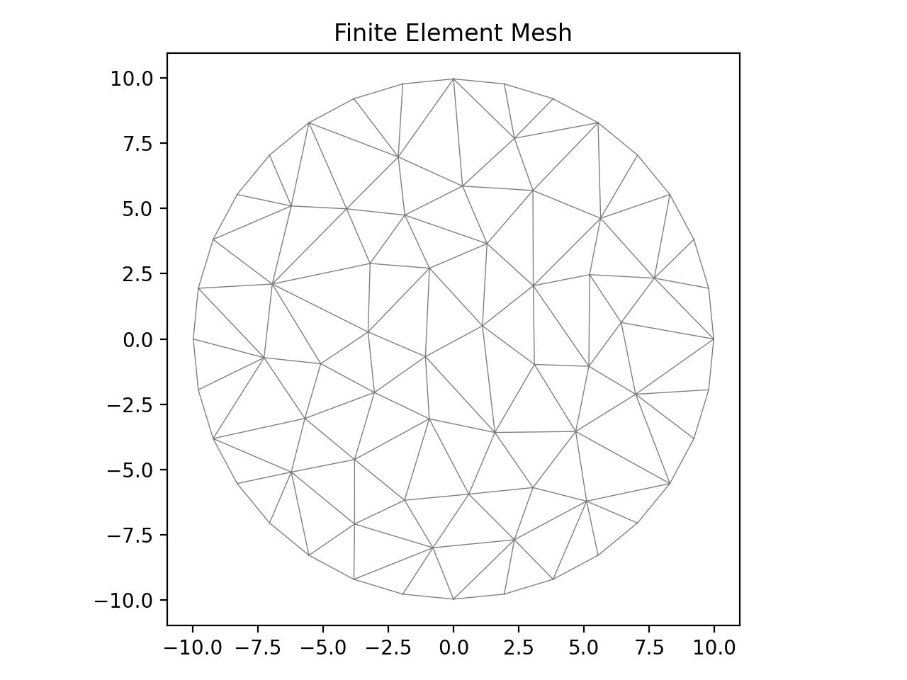
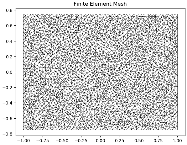
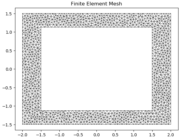
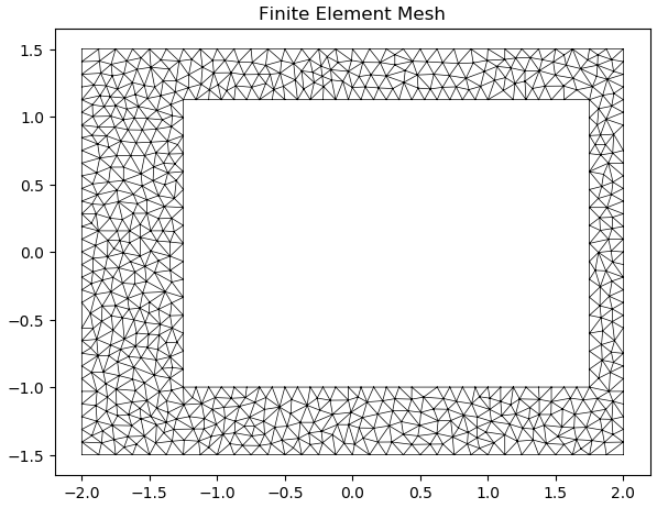
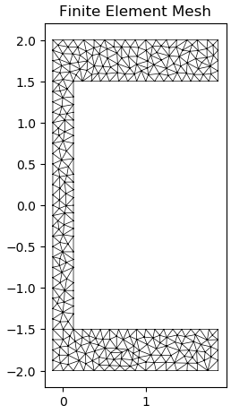
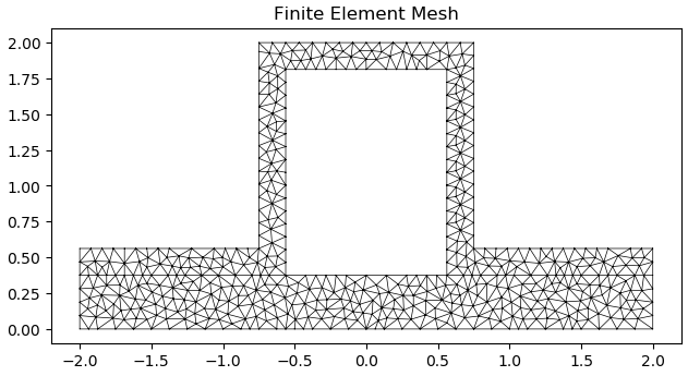
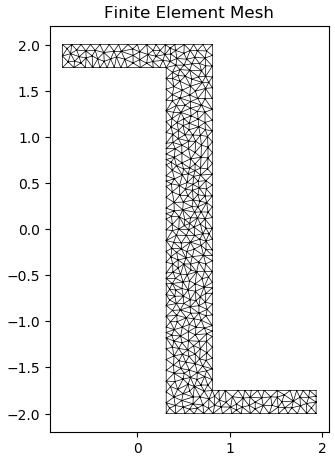
Creates a quadratic triangular mesh using the triangle module, which utilises the code
‘Triangle’, by Jonathan Shewchuk.
Parameters
points (list[list[int, int]]) – List of points (x, y) defining the vertices of the cross-section
facets – List of point index pairs (p1, p2) defining the edges of the cross-section
holes (list[list[float, float]]) – List of points (x, y) defining the locations of holes within the cross-section.
If there are no holes, provide an empty list [].
control_points (list[list[float, float]]) – A list of points (x, y) that define different regions of the
cross-section. A control point is an arbitrary point within a region enclosed by facets.
mesh_sizes (list[float]) – List of maximum element areas for each region defined by a control point
coarse (bool) – If set to True, will create a coarse mesh (no area or quality
constraints)
Load a Rhino .3dm file and import the single surface planer breps.
Parameters
r3dm_filepath (pathlib.Path or string) – File path to the rhino .3dm file.
kwargs – See below.
Raises
RuntimeError – A RuntimeError is raised if no polygons are found in the file.
This is dependent on the keyword arguments.
Try adjusting the keyword arguments if this error is raised.
Returns
List of Polygons found in the file.
Return type
List[shapely.geometry.Polygon]
Keyword Arguments
refine_num (int,optional) –
Bézier curve interpolation number. In Rhino a surface’s edges are nurb based curves.
Shapely does not support nurbs, so the individual Bézier curves are interpolated using straight lines.
This parameter sets the number of straight lines used in the interpolation.
Default is 1.
vec1 (numpy.ndarray,optional) –
A 3d vector in the Shapely plane. Rhino is a 3D geometry environment.
Shapely is a 2D geometric library.
Thus a 2D plane needs to be defined in Rhino that represents the Shapely coordinate system.
vec1 represents the 1st vector of this plane. It will be used as Shapely’s x direction.
Default is [1,0,0].
vec2 (numpy.ndarray,optional) –
Continuing from vec1, vec2 is another vector to define the Shapely plane.
It must not be [0,0,0] and it’s only requirement is that it is any vector in the Shapely plane (but not equal to vec1).
Default is [0,1,0].
plane_distance (float,optional) –
The distance to the Shapely plane.
Default is 0.
project (boolean,optional) –
Controls if the breps are projected onto the plane in the direction of the Shapley plane’s normal.
Default is True.
parallel (boolean,optional) –
Controls if only the rhino surfaces that have the same normal as the Shapely plane are yielded.
If true, all non parallel surfaces are filtered out.
Default is False.
RuntimeError – A RuntimeError is raised if no polygons are found in the encoding.
This is dependent on the keyword arguments.
Try adjusting the keyword arguments if this error is raised.
Returns
The Polygons found in the encoding string.
Return type
shapely.geometry.Polygon
Keyword Arguments
refine_num (int,optional) –
Bézier curve interpolation number. In Rhino a surface’s edges are nurb based curves.
Shapely does not support nurbs, so the individual Bézier curves are interpolated using straight lines.
This parameter sets the number of straight lines used in the interpolation.
Default is 1.
vec1 (numpy.ndarray,optional) –
A 3d vector in the Shapely plane. Rhino is a 3D geometry environment.
Shapely is a 2D geometric library.
Thus a 2D plane needs to be defined in Rhino that represents the Shapely coordinate system.
vec1 represents the 1st vector of this plane. It will be used as Shapely’s x direction.
Default is [1,0,0].
vec2 (numpy.ndarray,optional) –
Continuing from vec1, vec2 is another vector to define the Shapely plane.
It must not be [0,0,0] and it’s only requirement is that it is any vector in the Shapely plane (but not equal to vec1).
Default is [0,1,0].
plane_distance (float,optional) –
The distance to the Shapely plane.
Default is 0.
project (boolean,optional) –
Controls if the breps are projected onto the plane in the direction of the Shapley plane’s normal.
Default is True.
parallel (boolean,optional) –
Controls if only the rhino surfaces that have the same normal as the Shapely plane are yielded.
If true, all non parallel surfaces are filtered out.
Default is False.
Return a LineString of a line that contains ‘point_on_line’ in the direction of ‘unit_vector’
bounded by ‘bounds’.
‘bounds’ is a tuple of float containing a max ordinate and min ordinate.
Returns tuple of two lists representing the list of Polygons in ‘polys’ on the “top” side of ‘line’ and the
list of Polygons on the “bottom” side of the ‘line’ after the original geometry has been split by ‘line’.
The 0-th tuple element is the “top” polygons and the 1-st element is the “bottom” polygons.
In the event that ‘line’ is a perfectly vertical line, the “top” polys are the polygons on the “right” of the
‘line’ and the “bottom” polys are the polygons on the “left” of the ‘line’.
Returns a tuple representing the values of “m” and “b” from
for a line that is perpendicular to ‘m_slope’ and contains the
‘point_on_line’, which represents an (x, y) coordinate.
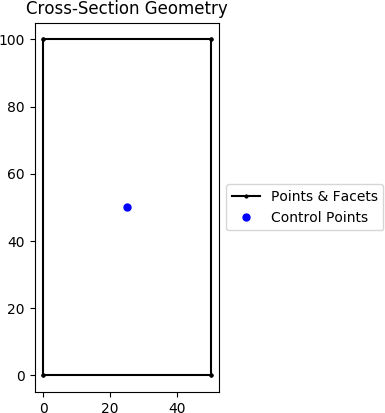
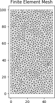
Constructs a rectangular section with the bottom left corner at the origin (0, 0), with
depth d and width b.
Parameters
d (float) – Depth (y) of the rectangle
b (float) – Width (x) of the rectangle
Optional[sectionproperties.pre.pre.Material] – Material to associate with this geometry
The following example creates a rectangular cross-section with a depth of 100 and width of 50,
and generates a mesh with a maximum triangular area of 5:
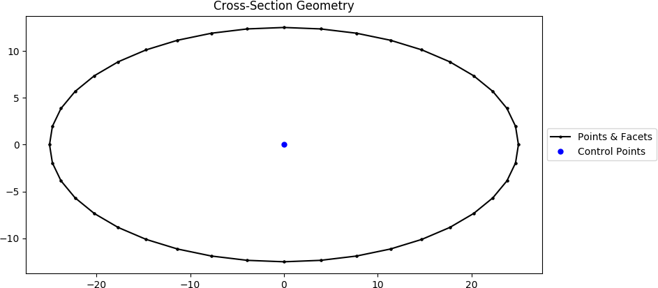
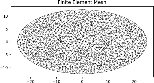
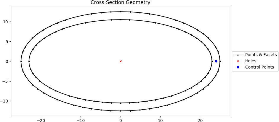
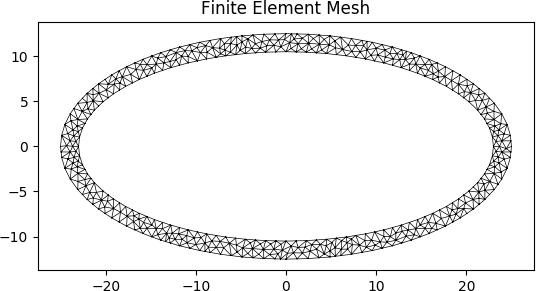
Constructs a solid ellipse centered at the origin (0, 0) with vertical diameter d_y and
horizontal diameter d_x, using n points to construct the ellipse.
Parameters
d_y (float) – Diameter of the ellipse in the y-dimension
d_x (float) – Diameter of the ellipse in the x-dimension
n (int) – Number of points discretising the ellipse
Optional[sectionproperties.pre.pre.Material] – Material to associate with this geometry
The following example creates an elliptical cross-section with a vertical diameter of 25 and
horizontal diameter of 50, with 40 points, and generates a mesh with a maximum triangular area
of 1.0:
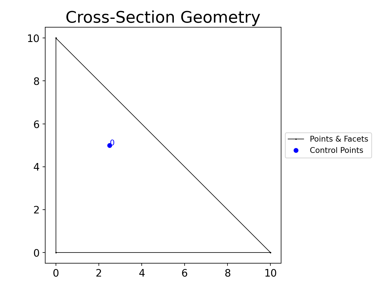
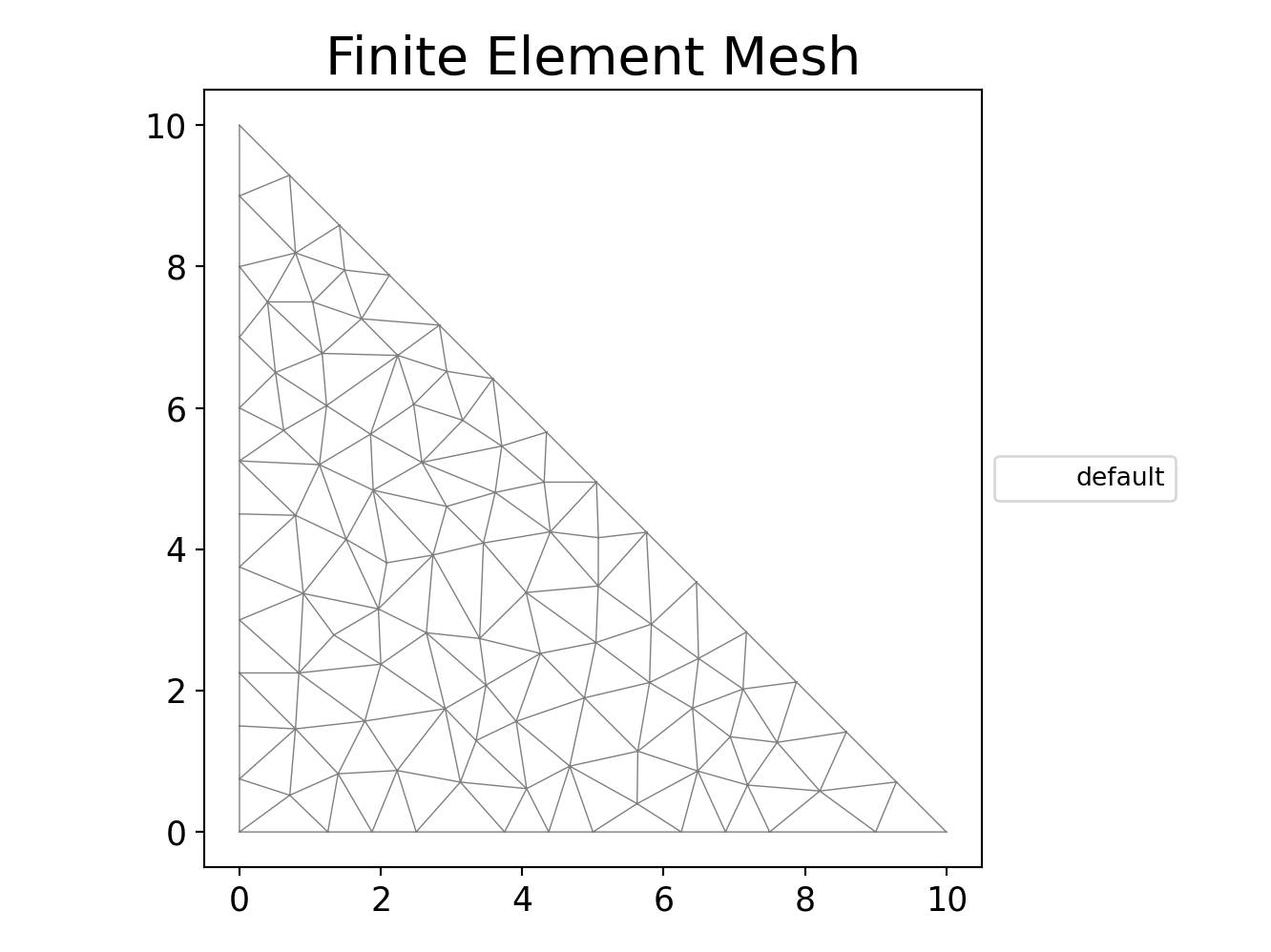
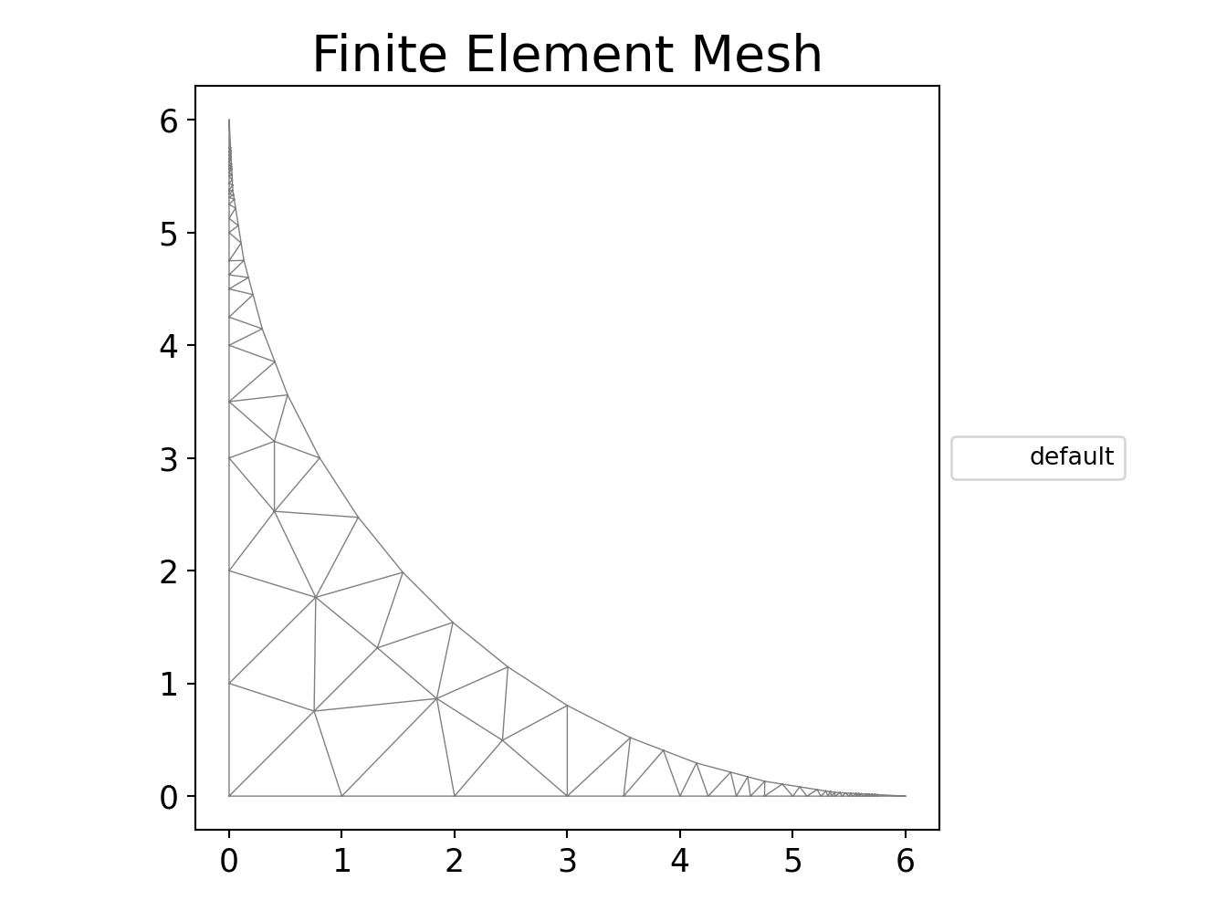
Constructs a right angled triangle with points (0, 0), (b, 0), (0, h).
Parameters
b (float) – Base length of triangle
h (float) – Height of triangle
Optional[sectionproperties.pre.pre.Material] – Material to associate with this geometry
The following example creates a triangular cross-section with a base width of 10 and height of
10, and generates a mesh with a maximum triangular area of 0.5:
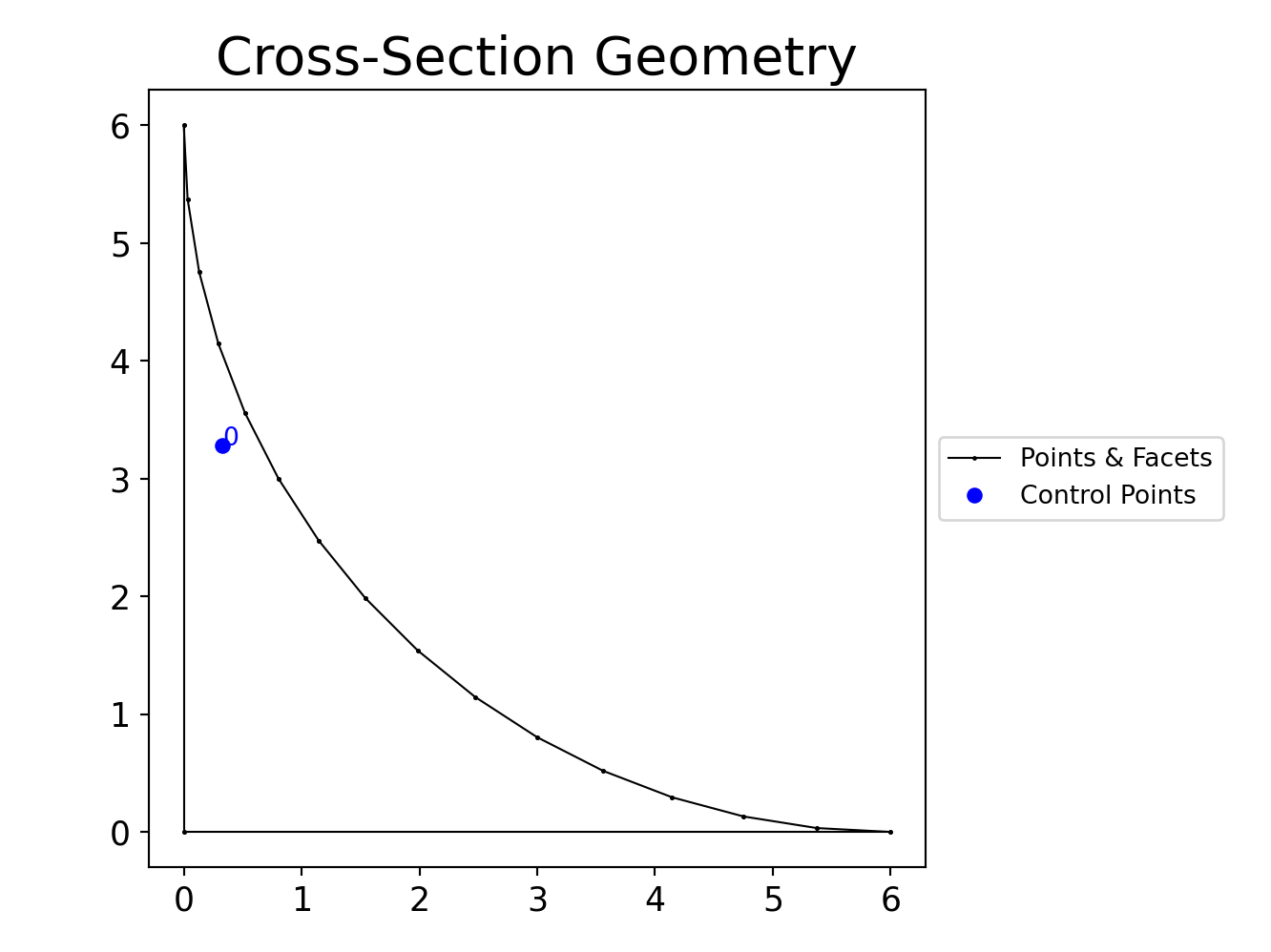
Constructs a right angled isosceles triangle with points (0, 0), (b, 0), (0, h) and a
concave radius on the hypotenuse.
Parameters
b (float) – Base length of triangle
n_r (int) – Number of points discretising the radius
Optional[sectionproperties.pre.pre.Material] – Material to associate with this geometry
The following example creates a triangular radius cross-section with a base width of 6, using
n_r points to construct the radius, and generates a mesh with a maximum triangular area of
0.5:
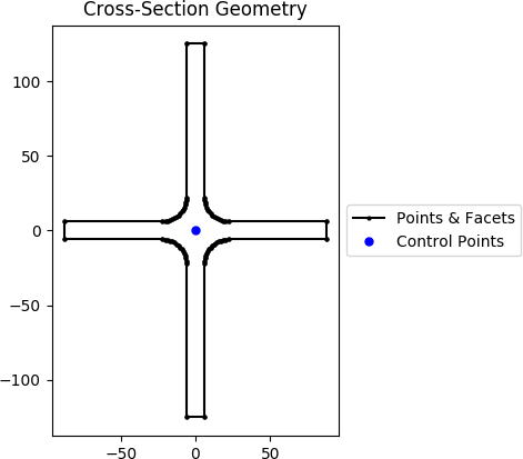
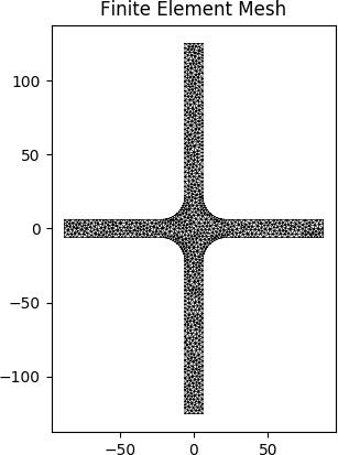
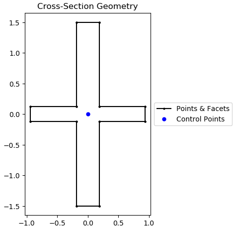
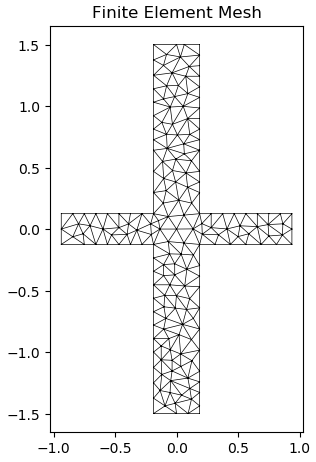
Constructs a cruciform section centered at the origin (0, 0), with depth d, width b,
thickness t and root radius r, using n_r points to construct the root radius.
Parameters
d (float) – Depth of the cruciform section
b (float) – Width of the cruciform section
t (float) – Thickness of the cruciform section
r (float) – Root radius of the cruciform section
n_r (int) – Number of points discretising the root radius
Optional[sectionproperties.pre.pre.Material] – Material to associate with this geometry
The following example creates a cruciform section with a depth of 250, a width of 175, a
thickness of 12 and a root radius of 16, using 16 points to discretise the radius. A mesh is
generated with a maximum triangular area of 5.0:
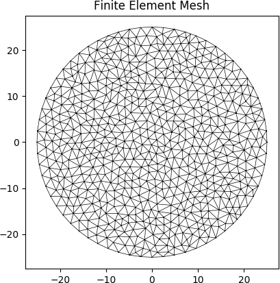
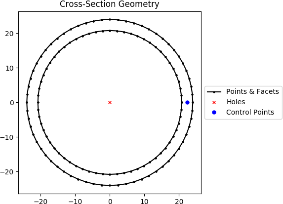
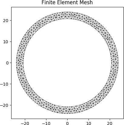
Constructs a circular hollow section (CHS) centered at the origin (0, 0), with diameter d and
thickness t, using n points to construct the inner and outer circles.
Parameters
d (float) – Outer diameter of the CHS
t (float) – Thickness of the CHS
n (int) – Number of points discretising the inner and outer circles
Optional[sectionproperties.pre.pre.Material] – Material to associate with this geometry
The following example creates a CHS discretised with 64 points, with a diameter of 48 and
thickness of 3.2, and generates a mesh with a maximum triangular area of 1.0:
Constructs an elliptical hollow section (EHS) centered at the origin (0, 0), with outer vertical
diameter d_y, outer horizontal diameter d_x, and thickness t, using n points to
construct the inner and outer ellipses.
Parameters
d_y (float) – Diameter of the ellipse in the y-dimension
d_x (float) – Diameter of the ellipse in the x-dimension
t (float) – Thickness of the EHS
n (int) – Number of points discretising the inner and outer ellipses
Optional[sectionproperties.pre.pre.Material] – Material to associate with this geometry
The following example creates a EHS discretised with 30 points, with a outer vertical diameter
of 25, outer horizontal diameter of 50, and thickness of 2.0, and generates a mesh with a
maximum triangular area of 0.5:
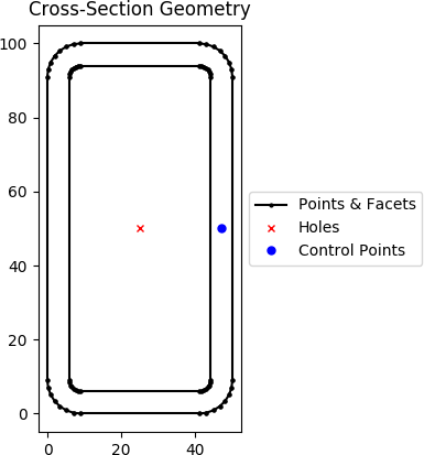
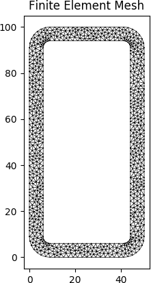
Constructs a rectangular hollow section (RHS) centered at (b/2, d/2), with depth d, width b,
thickness t and outer radius r_out, using n_r points to construct the inner and outer
radii. If the outer radius is less than the thickness of the RHS, the inner radius is set to
zero.
Parameters
d (float) – Depth of the RHS
b (float) – Width of the RHS
t (float) – Thickness of the RHS
r_out (float) – Outer radius of the RHS
n_r (int) – Number of points discretising the inner and outer radii
Optional[sectionproperties.pre.pre.Material] – Material to associate with this geometry
The following example creates an RHS with a depth of 100, a width of 50, a thickness of 6 and
an outer radius of 9, using 8 points to discretise the inner and outer radii. A mesh is
generated with a maximum triangular area of 2.0:
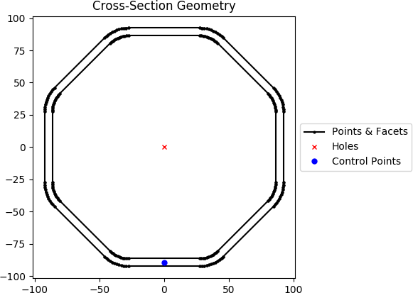
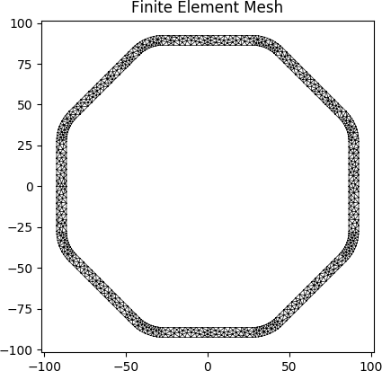
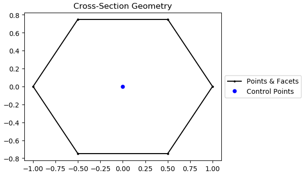
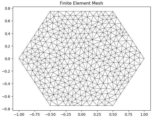
Constructs a regular hollow polygon section centered at (0, 0), with a pitch circle
diameter of bounding polygon d, thickness t, number of sides n_sides and an optional
inner radius r_in, using n_r points to construct the inner and outer radii (if radii is
specified).
Parameters
d (float) – Pitch circle diameter of the outer bounding polygon (i.e. diameter of circle
that passes through all vertices of the outer polygon)
t (float) – Thickness of the polygon section wall
r_in (float) – Inner radius of the polygon corners. By default, if not specified, a polygon
with no corner radii is generated.
n_r (int) – Number of points discretising the inner and outer radii, ignored if no inner
radii is specified
rot (float) – Initial counterclockwise rotation in degrees. By default bottom face is
aligned with x axis.
Optional[sectionproperties.pre.pre.Material] – Material to associate with this geometry
Raises
Exception – Number of sides in polygon must be greater than or equal to 3
The following example creates an Octagonal section (8 sides) with a diameter of 200, a
thickness of 6 and an inner radius of 20, using 12 points to discretise the inner and outer
radii. A mesh is generated with a maximum triangular area of 5:
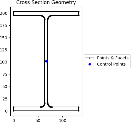
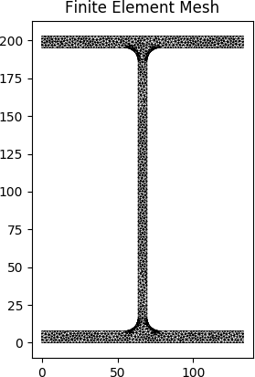
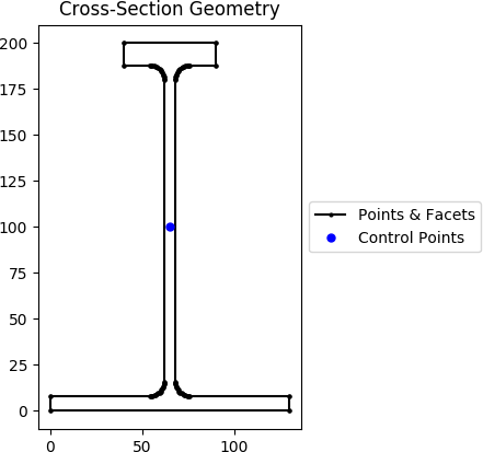
Constructs an I Section centered at (b/2, d/2), with depth d, width b, flange
thickness t_f, web thickness t_w, and root radius r, using n_r points to construct the
root radius.
Parameters
d (float) – Depth of the I Section
b (float) – Width of the I Section
t_f (float) – Flange thickness of the I Section
t_w (float) – Web thickness of the I Section
r (float) – Root radius of the I Section
n_r (int) – Number of points discretising the root radius
Optional[sectionproperties.pre.pre.Material] – Material to associate with this geometry
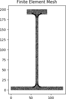
The following example creates an I Section with a depth of 203, a width of 133, a flange
thickness of 7.8, a web thickness of 5.8 and a root radius of 8.9, using 16 points to
discretise the root radius. A mesh is generated with a maximum triangular area of 3.0:
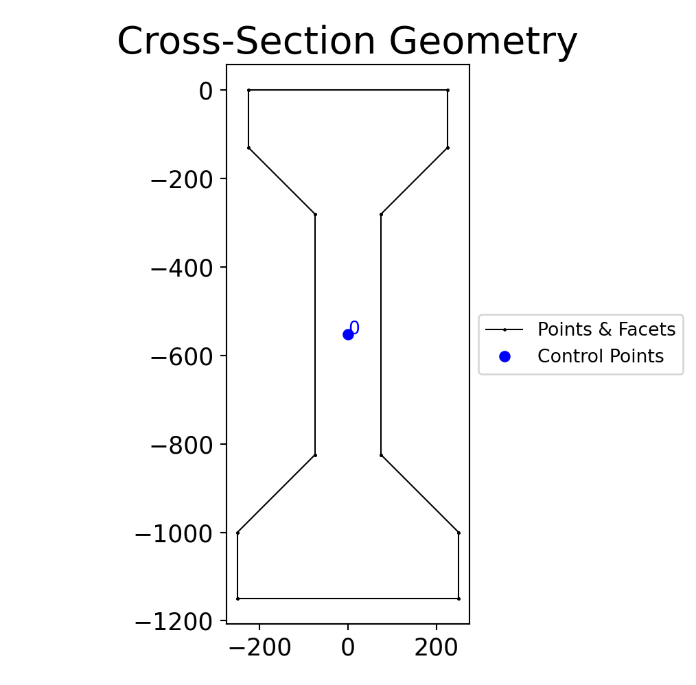
Constructs a monosymmetric I Section centered at (max(b_t, b_b)/2, d/2), with depth d,
top flange width b_t, bottom flange width b_b, top flange thickness t_ft, top flange
thickness t_fb, web thickness t_w, and root radius r, using n_r points to construct the
root radius.
Parameters
d (float) – Depth of the I Section
b_t (float) – Top flange width
b_b (float) – Bottom flange width
t_ft (float) – Top flange thickness of the I Section
t_fb (float) – Bottom flange thickness of the I Section
t_w (float) – Web thickness of the I Section
r (float) – Root radius of the I Section
n_r (int) – Number of points discretising the root radius
Optional[sectionproperties.pre.pre.Material] – Material to associate with this geometry
The following example creates a monosymmetric I Section with a depth of 200, a top flange width
of 50, a top flange thickness of 12, a bottom flange width of 130, a bottom flange thickness of
8, a web thickness of 6 and a root radius of 8, using 16 points to discretise the root radius.
A mesh is generated with a maximum triangular area of 3.0:
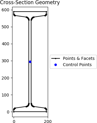
Constructs a Tapered Flange I Section centered at (b/2, d/2), with depth d, width b,
mid-flange thickness t_f, web thickness t_w, root radius r_r, flange radius r_f and
flange angle alpha, using n_r points to construct the radii.
Parameters
d (float) – Depth of the Tapered Flange I Section
b (float) – Width of the Tapered Flange I Section
t_f (float) – Mid-flange thickness of the Tapered Flange I Section (measured at the point
equidistant from the face of the web to the edge of the flange)
t_w (float) – Web thickness of the Tapered Flange I Section
r_r (float) – Root radius of the Tapered Flange I Section
r_f (float) – Flange radius of the Tapered Flange I Section
alpha (float) – Flange angle of the Tapered Flange I Section (degrees)
n_r (int) – Number of points discretising the radii
Optional[sectionproperties.pre.pre.Material] – Material to associate with this geometry
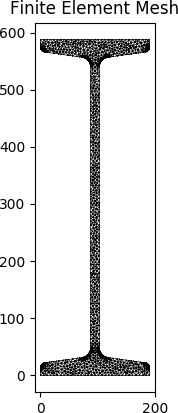
The following example creates a Tapered Flange I Section with a depth of 588, a width of 191, a
mid-flange thickness of 27.2, a web thickness of 15.2, a root radius of 17.8, a flange radius
of 8.9 and a flange angle of 8°, using 16 points to discretise the radii. A mesh is generated
with a maximum triangular area of 20.0:
Constructs a parallel-flange channel (PFC) section with the bottom left corner at the origin (0, 0), with depth d,
width b, flange thickness t_f, web thickness t_w and root radius r, using n_r points
to construct the root radius.
Parameters
d (float) – Depth of the PFC section
b (float) – Width of the PFC section
t_f (float) – Flange thickness of the PFC section
t_w (float) – Web thickness of the PFC section
r (float) – Root radius of the PFC section
n_r (int) – Number of points discretising the root radius
shift (list[float, float]) – Vector that shifts the cross-section by (x, y)
Optional[sectionproperties.pre.pre.Material] – Material to associate with this geometry
The following example creates a PFC section with a depth of 250, a width of 90, a flange
thickness of 15, a web thickness of 8 and a root radius of 12, using 8 points to discretise the
root radius. A mesh is generated with a maximum triangular area of 5.0:
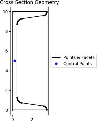
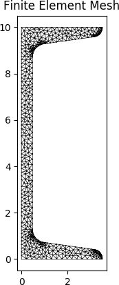
Constructs a Tapered Flange Channel section with the bottom left corner at the origin
(0, 0), with depth d, width b, mid-flange thickness t_f, web thickness t_w, root
radius r_r, flange radius r_f and flange angle alpha, using n_r points to construct the
radii.
Parameters
d (float) – Depth of the Tapered Flange Channel section
b (float) – Width of the Tapered Flange Channel section
t_f (float) – Mid-flange thickness of the Tapered Flange Channel section (measured at the
point equidistant from the face of the web to the edge of the flange)
t_w (float) – Web thickness of the Tapered Flange Channel section
r_r (float) – Root radius of the Tapered Flange Channel section
r_f (float) – Flange radius of the Tapered Flange Channel section
alpha (float) – Flange angle of the Tapered Flange Channel section (degrees)
n_r (int) – Number of points discretising the radii
Optional[sectionproperties.pre.pre.Material] – Material to associate with this geometry
The following example creates a Tapered Flange Channel section with a depth of 10, a width of
3.5, a mid-flange thickness of 0.575, a web thickness of 0.475, a root radius of 0.575, a
flange radius of 0.4 and a flange angle of 8°, using 16 points to discretise the radii. A mesh
is generated with a maximum triangular area of 0.02:
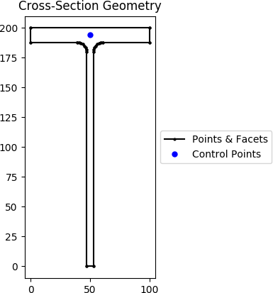
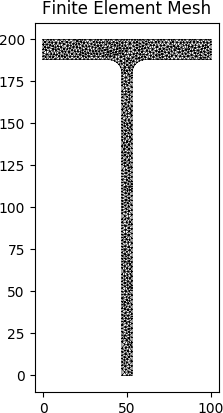
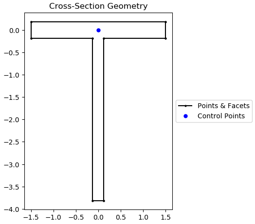
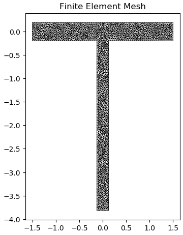
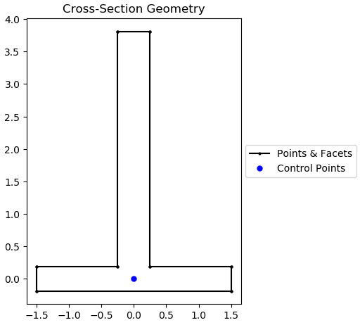
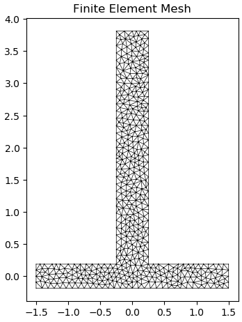
Constructs a Tee section with the top left corner at (0, d), with depth d, width b,
flange thickness t_f, web thickness t_w and root radius r, using n_r points to
construct the root radius.
Parameters
d (float) – Depth of the Tee section
b (float) – Width of the Tee section
t_f (float) – Flange thickness of the Tee section
t_w (float) – Web thickness of the Tee section
r (float) – Root radius of the Tee section
n_r (int) – Number of points discretising the root radius
Optional[sectionproperties.pre.pre.Material] – Material to associate with this geometry
The following example creates a Tee section with a depth of 200, a width of 100, a flange
thickness of 12, a web thickness of 6 and a root radius of 8, using 8 points to discretise the
root radius. A mesh is generated with a maximum triangular area of 3.0:
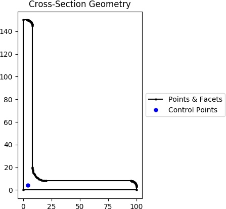
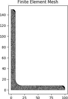
Constructs an angle section with the bottom left corner at the origin (0, 0), with depth
d, width b, thickness t, root radius r_r and toe radius r_t, using n_r points to
construct the radii.
Parameters
d (float) – Depth of the angle section
b (float) – Width of the angle section
t (float) – Thickness of the angle section
r_r (float) – Root radius of the angle section
r_t (float) – Toe radius of the angle section
n_r (int) – Number of points discretising the radii
Optional[sectionproperties.pre.pre.Material] – Material to associate with this geometry
The following example creates an angle section with a depth of 150, a width of 100, a thickness
of 8, a root radius of 12 and a toe radius of 5, using 16 points to discretise the radii. A
mesh is generated with a maximum triangular area of 2.0:
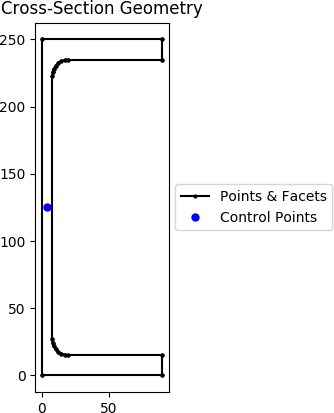
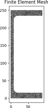
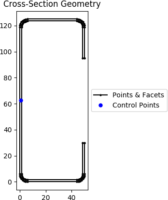
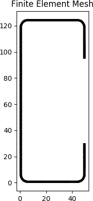
Constructs a Cee section (typical of cold-formed steel) with the bottom left corner at the
origin (0, 0), with depth d, width b, lip l, thickness t and outer radius r_out,
using n_r points to construct the radius. If the outer radius is less than the thickness
of the Cee Section, the inner radius is set to zero.
Parameters
d (float) – Depth of the Cee section
b (float) – Width of the Cee section
l (float) – Lip of the Cee section
t (float) – Thickness of the Cee section
r_out (float) – Outer radius of the Cee section
n_r (int) – Number of points discretising the outer radius
Optional[sectionproperties.pre.pre.Material] – Material to associate with this geometry
Raises
Exception – Lip length must be greater than the outer radius
The following example creates a Cee section with a depth of 125, a width of 50, a lip of 30, a
thickness of 1.5 and an outer radius of 6, using 8 points to discretise the radius. A mesh is
generated with a maximum triangular area of 0.25:
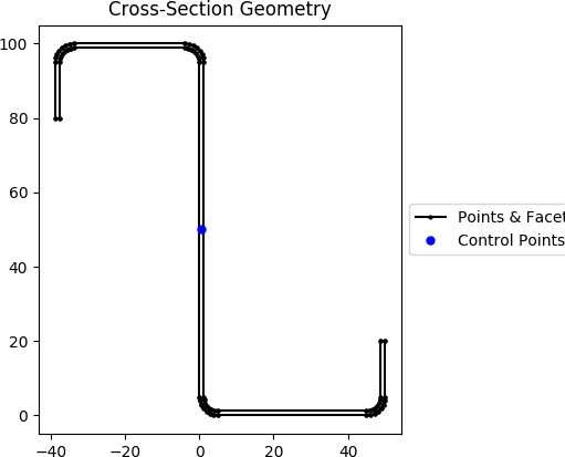
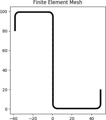
Constructs a zed section with the bottom left corner at the origin (0, 0), with depth d,
left flange width b_l, right flange width b_r, lip l, thickness t and outer radius
r_out, using n_r points to construct the radius. If the outer radius is less than the
thickness of the Zed Section, the inner radius is set to zero.
Parameters
d (float) – Depth of the zed section
b_l (float) – Left flange width of the Zed section
b_r (float) – Right flange width of the Zed section
l (float) – Lip of the Zed section
t (float) – Thickness of the Zed section
r_out (float) – Outer radius of the Zed section
n_r (int) – Number of points discretising the outer radius
Optional[sectionproperties.pre.pre.Material] – Material to associate with this geometry
The following example creates a zed section with a depth of 100, a left flange width of 40, a
right flange width of 50, a lip of 20, a thickness of 1.2 and an outer radius of 5, using 8
points to discretise the radius. A mesh is generated with a maximum triangular area of 0.15:
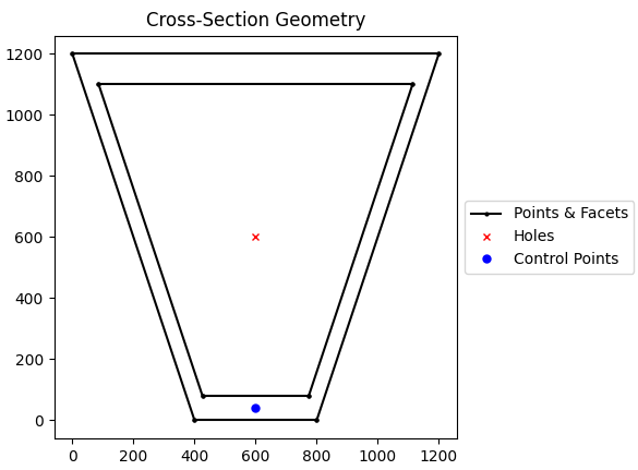
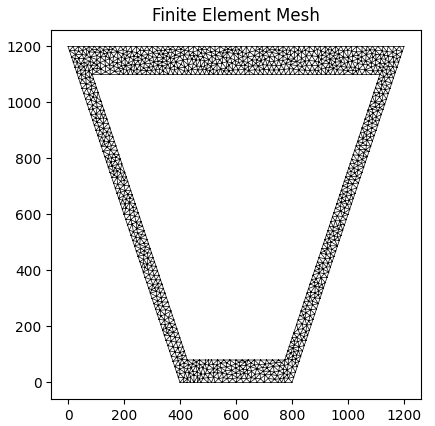
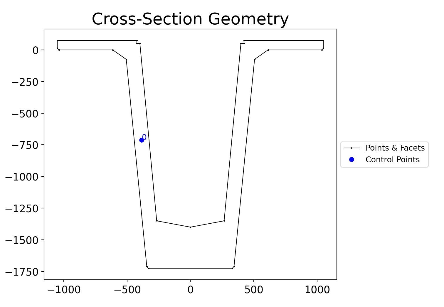
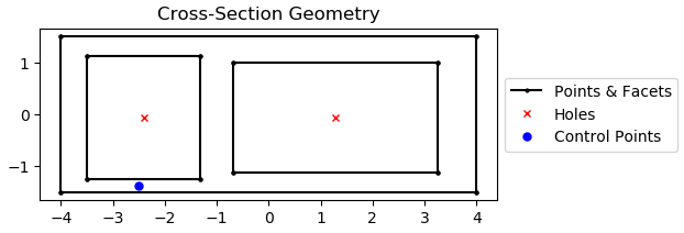
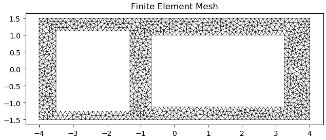
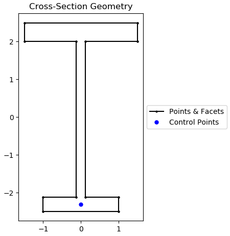
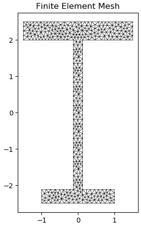
Constructs a box girder section centered at at (max(b_t, b_b)/2, d/2), with depth d, top
width b_t, bottom width b_b, top flange thickness t_ft, bottom flange thickness t_fb
and web thickness t_w.
Parameters
d (float) – Depth of the Box Girder section
b_t (float) – Top width of the Box Girder section
b_b (float) – Bottom width of the Box Girder section
t_ft (float) – Top flange thickness of the Box Girder section
t_fb (float) – Bottom flange thickness of the Box Girder section
t_w (float) – Web thickness of the Box Girder section
The following example creates a Box Girder section with a depth of 1200, a top width of 1200, a
bottom width of 400, a top flange thickness of 16, a bottom flange thickness of 12 and a web
thickness of 8. A mesh is generated with a maximum triangular area of 5.0:
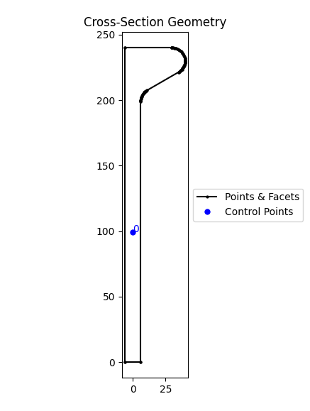
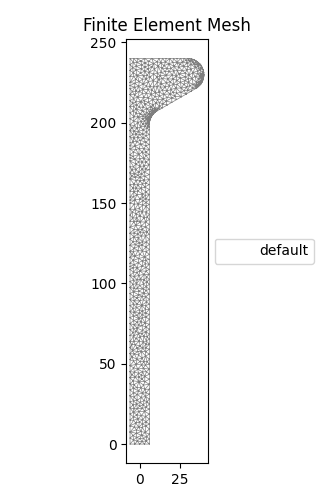
Constructs a bulb section with the bottom left corner at the point
(-t / 2, 0), with depth d, bulb depth d_b, bulb width b, web thickness t
and radius r, using n_r points to construct the radius.
Parameters
d (float) – Depth of the section
b (float) – Bulb width
t (float) – Web thickness
r (float) – Bulb radius
d_b (float) – Depth of the bulb (automatically calculated for standard sections,
if provided the section may have sharp edges)
n_r (int) – Number of points discretising the radius
Optional[sectionproperties.pre.pre.Material] – Material to associate with
this geometry
The following example creates a bulb section with a depth of 240, a width of 34, a
web thickness of 12 and a bulb radius of 16, using 16 points to discretise the
radius. A mesh is generated with a maximum triangular area of 5.0:
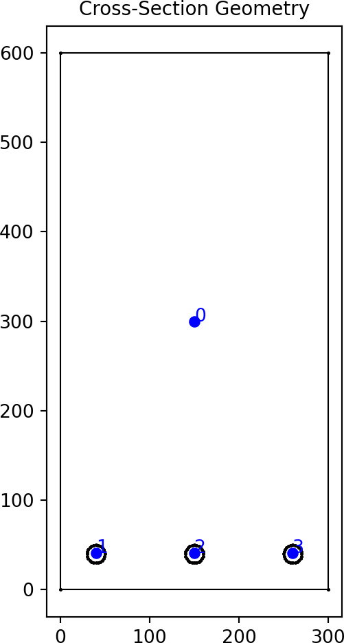
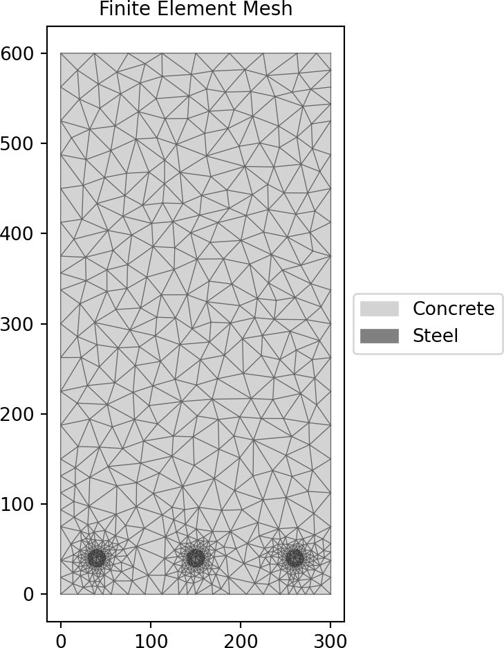
Constructs a concrete rectangular section of width b and depth d, with
n_top top steel bars of diameter dia_top, n_bot bottom steel bars of diameter
dia_bot, n_side left & right side steel bars of diameter dia_side discretised
with n_circle points with equal side and top/bottom cover to the steel.
Parameters
b (float) – Concrete section width
d (float) – Concrete section depth
dia_top (float) – Diameter of the top steel reinforcing bars
n_top (int) – Number of top steel reinforcing bars
dia_bot (float) – Diameter of the bottom steel reinforcing bars
n_bot (int) – Number of bottom steel reinforcing bars
n_circle (int) – Number of points discretising the steel reinforcing bars
cover (float) – Side and bottom cover to the steel reinforcing bars
dia_side (float) – If provided, diameter of the side steel reinforcing bars
n_side (int) – If provided, number of side bars either side of the section
area_top (float) – If provided, constructs top reinforcing bars based on their
area rather than diameter (prevents the underestimation of steel area due to
circle discretisation)
area_bot (float) – If provided, constructs bottom reinforcing bars based on
their area rather than diameter (prevents the underestimation of steel area due
to circle discretisation)
area_side (float) – If provided, constructs side reinforcing bars based on
their area rather than diameter (prevents the underestimation of steel area due
to circle discretisation)
conc_mat – Material to associate with the concrete
steel_mat – Material to associate with the steel
Raises
ValueError – If the number of bars is not greater than or equal to 2 in an
active layer
The following example creates a 600D x 300W concrete beam with 3N20 bottom steel
reinforcing bars and 30 mm cover:
Constructs a concrete rectangular section of width b and depth d, with
steel bar reinforcing organized as an n_bars_b by n_bars_d array, discretised
with n_circle points with equal sides and top/bottom cover to the steel which
is taken as the clear cover (edge of bar to edge of concrete).
Parameters
b (float) – Concrete section width, parallel to the x-axis
d (float) – Concrete section depth, parallel to the y-axis
cover (float) – Clear cover, calculated as distance from edge of reinforcing bar to edge of section.
n_bars_b (int) – Number of bars placed across the width of the section, minimum 2.
n_bars_d (int) – Number of bars placed across the depth of the section, minimum 2.
dia_bar (float) – Diameter of reinforcing bars. Used for calculating bar placement and,
optionally, for calculating the bar area for section capacity calculations.
bar_area (float) – Area of reinforcing bars. Used for section capacity calculations.
If not provided, then dia_bar will be used to calculate the bar area.
filled (bool) – When True, will populate the concrete section with an equally
spaced 2D array of reinforcing bars numbering ‘n_bars_b’ by ‘n_bars_d’.
When False, only the bars around the perimeter of the array will be present.
n_circle (int) – The number of points used to discretize the circle of the reinforcing
bars. The bars themselves will have an exact area of ‘bar_area’ regardless of the
number of points used in the circle. Useful for making the reinforcing bars look
more circular when plotting the concrete section.
Raises
ValueError – If the number of bars in either ‘n_bars_b’ or ‘n_bars_d’ is not greater
than or equal to 2.
The following example creates a 600D x 300W concrete column with 25 mm diameter
reinforcing bars each with 500 mm**2 area and 35 mm cover in a 3x6 array without
the interior bars being filled:
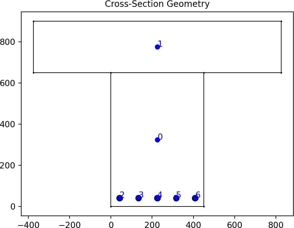
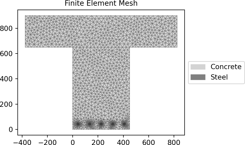
Constructs a concrete tee section of width b, depth d, flange width b_f
and flange depth d_f, with n_top top steel bars of diameter dia_top, n_bot
bottom steel bars of diameter dia_bot, discretised with n_circle points with
equal side and top/bottom cover to the steel.
Parameters
b (float) – Concrete section width
d (float) – Concrete section depth
b_f (float) – Concrete section flange width
d_f (float) – Concrete section flange depth
dia_top (float) – Diameter of the top steel reinforcing bars
n_top (int) – Number of top steel reinforcing bars
dia_bot (float) – Diameter of the bottom steel reinforcing bars
n_bot (int) – Number of bottom steel reinforcing bars
n_circle (int) – Number of points discretising the steel reinforcing bars
cover (float) – Side and bottom cover to the steel reinforcing bars
area_top (float) – If provided, constructs top reinforcing bars based on their
area rather than diameter (prevents the underestimation of steel area due to
circle discretisation)
area_bot (float) – If provided, constructs bottom reinforcing bars based on
their area rather than diameter (prevents the underestimation of steel area due
to circle discretisation)
conc_mat – Material to associatewith the concrete
steel_mat – Material toassociate with the steel
Raises
ValueErorr – If the number of bars is not greater than or equal to 2 in an
active layer
The following example creates a 900D x 450W concrete beam with a 1200W x 250D
flange, with 5N24 steel reinforcing bars and 30 mm cover:
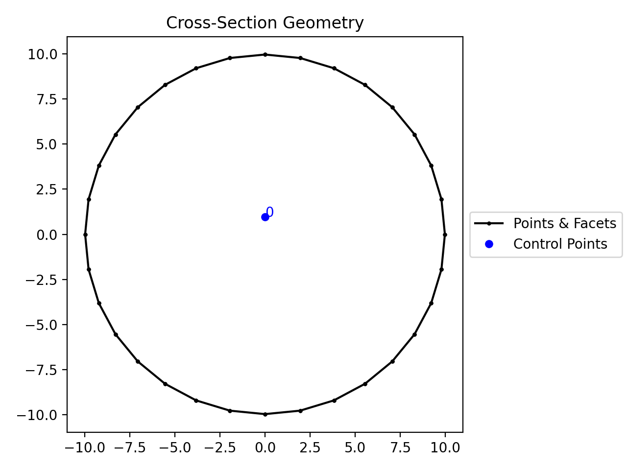
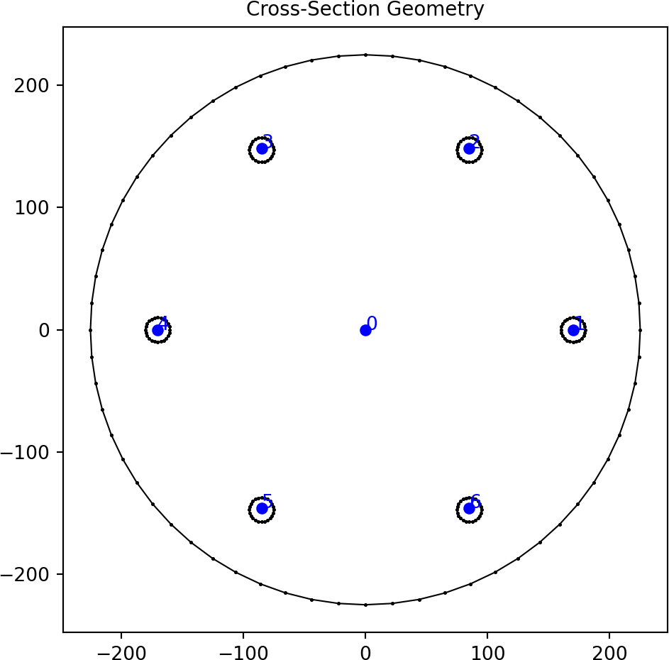
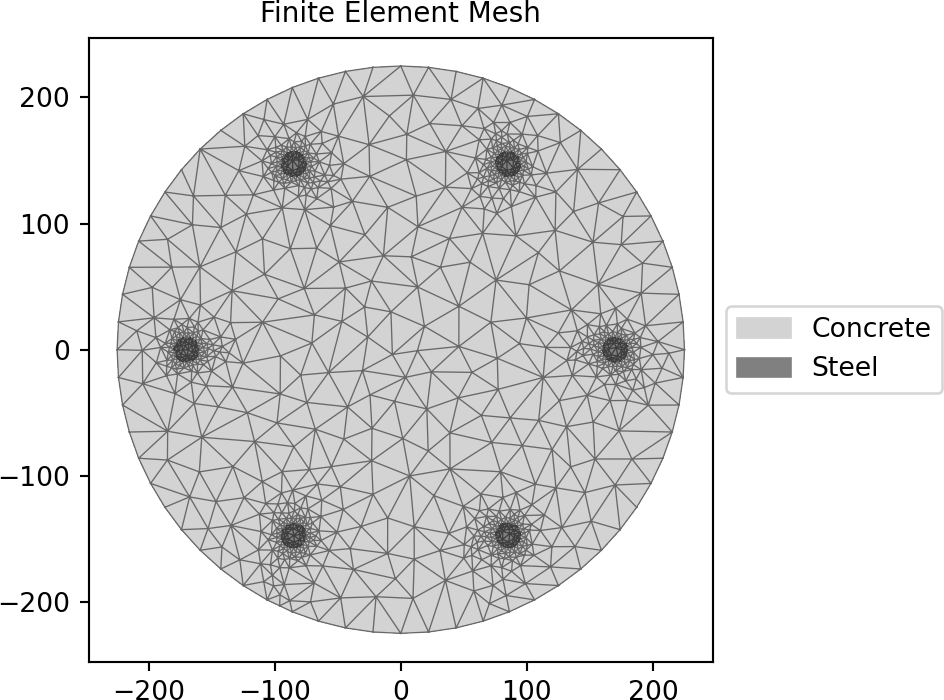
Constructs a concrete circular section of diameter d discretised with n
points, with n_bar steel bars of diameter dia, discretised with n_circle
points with equal side and bottom cover to the steel.
Parameters
d (float) – Concrete diameter
n (float) – Number of points discretising the concrete section
dia (float) – Diameter of the steel reinforcing bars
n_bar (int) – Number of steel reinforcing bars
n_circle (int) – Number of points discretising the steel reinforcing bars
cover (float) – Side and bottom cover to the steel reinforcing bars
area_conc (float) – If provided, constructs the concrete based on its area
rather than diameter (prevents the underestimation of concrete area due to
circle discretisation)
area_bar (float) – If provided, constructs reinforcing bars based on their area
rather than diameter (prevents the underestimation of steel area due to
conc_mat – Material to associate with the concrete
steel_mat – Material to associate with the steel
Raises
ValueErorr – If the number of bars is not greater than or equal to 2
The following example creates a 450DIA concrete column with with 6N20 steel
reinforcing bars and 45 mm cover:
Note that the properties are reported as modulusweighted properties (e.g. E.A) and can
be normalized to the reference material by dividing by that elastic modulus:
A_65=section.get_ea()/precast.elastic_modulus
The reported section centroids are already weighted.
Constructs a BAR section with the center at the origin (0, 0), with two parameters
defining dimensions. See Nastran documentation 12345 for definition of
parameters. Added by JohnDN90.
Parameters
DIM1 (float) – Width (x) of bar
DIM2 (float) – Depth (y) of bar
Optional[sectionproperties.pre.pre.Material] – Material to associate with this geometry
The following example creates a BAR cross-section with a depth of 1.5 and width of 2.0, and
generates a mesh with a maximum triangular area of 0.001:
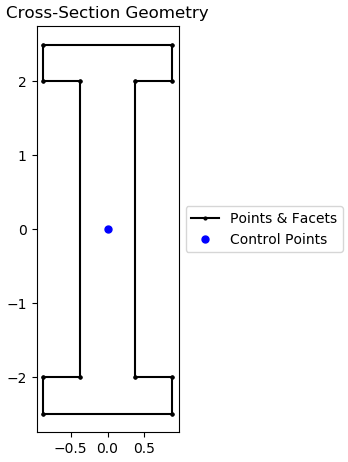
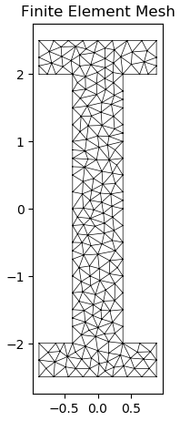
Constructs a BOX section with the center at the origin (0, 0), with four parameters
defining dimensions. See Nastran documentation 12345 for definition of
parameters. Added by JohnDN90.
Parameters
DIM1 (float) – Width (x) of box
DIM2 (float) – Depth (y) of box
DIM3 (float) – Thickness of box in y direction
DIM4 (float) – Thickness of box in x direction
Optional[sectionproperties.pre.pre.Material] – Material to associate with this geometry
The following example creates a BOX cross-section with a depth of 3.0 and width of 4.0, and
generates a mesh with a maximum triangular area of 0.001:
Constructs a BOX1 section with the center at the origin (0, 0), with six parameters
defining dimensions. See Nastran documentation 1234 for more details. Added by
JohnDN90.
Parameters
DIM1 (float) – Width (x) of box
DIM2 (float) – Depth (y) of box
DIM3 (float) – Thickness of top wall
DIM4 (float) – Thickness of bottom wall
DIM5 (float) – Thickness of left wall
DIM6 (float) – Thickness of right wall
Optional[sectionproperties.pre.pre.Material] – Material to associate with this geometry
The following example creates a BOX1 cross-section with a depth of 3.0 and width of 4.0, and
generates a mesh with a maximum triangular area of 0.007:
Constructs a CHAN (C-Channel) section with the web’s middle center at the origin (0, 0),
with four parameters defining dimensions. See Nastran documentation 1234 for
more details. Added by JohnDN90.
Parameters
DIM1 (float) – Width (x) of the CHAN-section
DIM2 (float) – Depth (y) of the CHAN-section
DIM3 (float) – Thickness of web (vertical portion)
DIM4 (float) – Thickness of flanges (top/bottom portion)
Optional[sectionproperties.pre.pre.Material] – Material to associate with this geometry
The following example creates a CHAN cross-section with a depth of 4.0 and width of 2.0, and
generates a mesh with a maximum triangular area of 0.008:
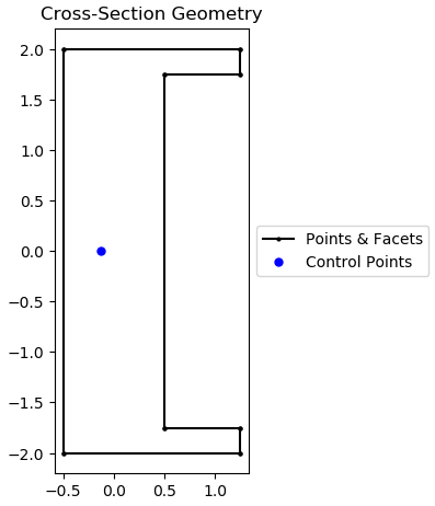
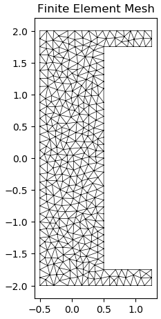
Constructs a CHAN1 (C-Channel) section with the web’s middle center at the origin (0, 0),
with four parameters defining dimensions. See Nastran documentation 1234 for
more details. Added by JohnDN90.
Parameters
DIM1 (float) – Width (x) of channels
DIM2 (float) – Thickness (x) of web
DIM3 (float) – Spacing between channels (length of web)
DIM4 (float) – Depth (y) of CHAN1-section
Optional[sectionproperties.pre.pre.Material] – Material to associate with this geometry
The following example creates a CHAN1 cross-section with a depth of 4.0 and width of 1.75, and
generates a mesh with a maximum triangular area of 0.01:
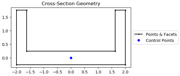
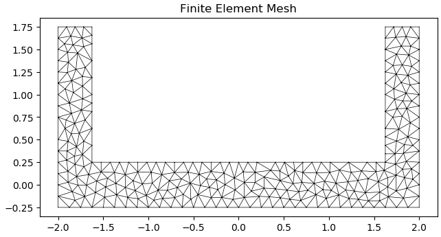
Constructs a CHAN2 (C-Channel) section with the bottom web’s middle center at the origin
(0, 0), with four parameters defining dimensions. See Nastran documentation 1234 for more details. Added by JohnDN90.
Parameters
DIM1 (float) – Thickness of channels
DIM2 (float) – Thickness of web
DIM3 (float) – Depth (y) of CHAN2-section
DIM4 (float) – Width (x) of CHAN2-section
Optional[sectionproperties.pre.pre.Material] – Material to associate with this geometry
The following example creates a CHAN2 cross-section with a depth of 2.0 and width of 4.0, and
generates a mesh with a maximum triangular area of 0.01:
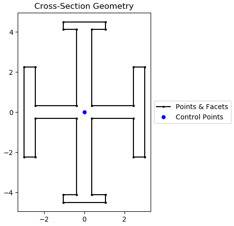
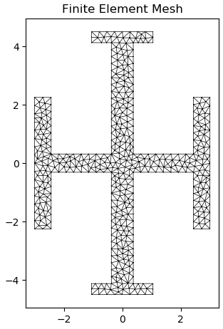
Constructs Nastran’s cruciform/cross section with the intersection’s middle center at the
origin (0, 0), with four parameters defining dimensions. See Nastran documentation 1234 for more details. Added by JohnDN90.
Parameters
DIM1 (float) – Twice the width of horizontal member protruding from the vertical center
member
DIM2 (float) – Thickness of the vertical member
DIM3 (float) – Depth (y) of the CROSS-section
DIM4 (float) – Thickness of the horizontal members
Optional[sectionproperties.pre.pre.Material] – Material to associate with this geometry
The following example creates a rectangular cross-section with a depth of 3.0 and width of
1.875, and generates a mesh with a maximum triangular area of 0.008:
Constructs a DBOX section with the center at the origin (0, 0), with ten parameters
defining dimensions. See MSC Nastran documentation 1 for more details. Added by JohnDN90.
Parameters
DIM1 (float) – Width (x) of the DBOX-section
DIM2 (float) – Depth (y) of the DBOX-section
DIM3 (float) – Width (x) of left-side box
DIM4 (float) – Thickness of left wall
DIM5 (float) – Thickness of center wall
DIM6 (float) – Thickness of right wall
DIM7 (float) – Thickness of top left wall
DIM8 (float) – Thickness of bottom left wall
DIM9 (float) – Thickness of top right wall
DIM10 (float) – Thickness of bottom right wall
Optional[sectionproperties.pre.pre.Material] – Material to associate with this geometry
The following example creates a DBOX cross-section with a depth of 3.0 and width of 8.0, and
generates a mesh with a maximum triangular area of 0.01:
Constructs a flanged cruciform/cross section with the intersection’s middle center at the
origin (0, 0), with eight parameters defining dimensions. Added by JohnDN90.
Parameters
DIM1 (float) – Depth (y) of flanged cruciform
DIM2 (float) – Width (x) of flanged cruciform
DIM3 (float) – Thickness of vertical web
DIM4 (float) – Thickness of horizontal web
DIM5 (float) – Length of flange attached to vertical web
DIM6 (float) – Thickness of flange attached to vertical web
DIM7 (float) – Length of flange attached to horizontal web
DIM8 (float) – Thickness of flange attached to horizontal web
Optional[sectionproperties.pre.pre.Material] – Material to associate with this geometry
The following example demonstrates the creation of a flanged cross section:
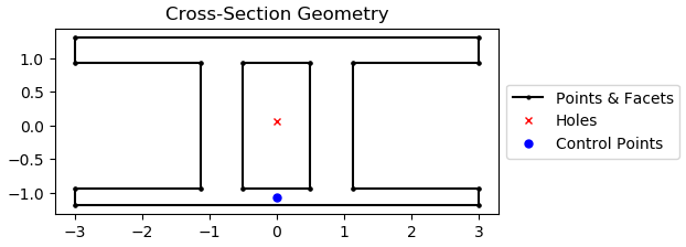
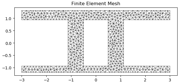
Constructs a GBOX section with the center at the origin (0, 0), with six parameters
defining dimensions. See ASTROS documentation 5 for more details. Added by JohnDN90.
Parameters
DIM1 (float) – Width (x) of the GBOX-section
DIM2 (float) – Depth (y) of the GBOX-section
DIM3 (float) – Thickness of top flange
DIM4 (float) – Thickness of bottom flange
DIM5 (float) – Thickness of webs
DIM6 (float) – Spacing between webs
Optional[sectionproperties.pre.pre.Material] – Material to associate with this geometry
The following example creates a GBOX cross-section with a depth of 2.5 and width of 6.0, and
generates a mesh with a maximum triangular area of 0.01:
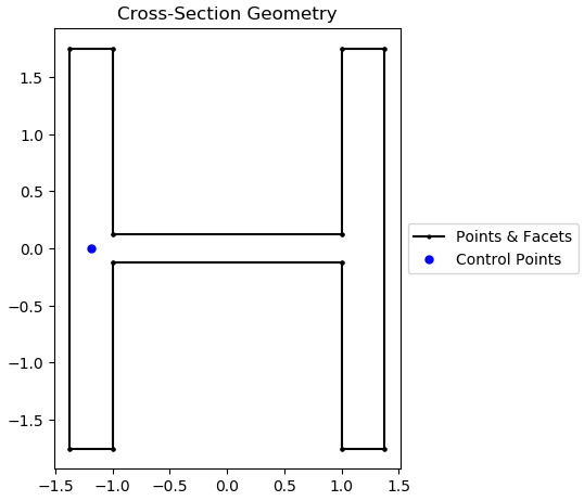
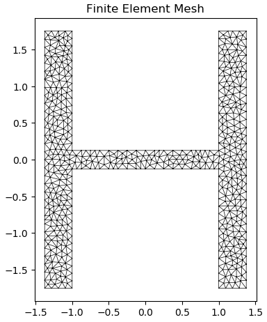
Constructs a H section with the middle web’s middle center at the origin (0, 0), with four
parameters defining dimensions. See Nastran documentation 1234 for more details.
Added by JohnDN90.
Parameters
DIM1 (float) – Spacing between vertical flanges (length of web)
DIM2 (float) – Twice the thickness of the vertical flanges
DIM3 (float) – Depth (y) of the H-section
DIM4 (float) – Thickness of the middle web
Optional[sectionproperties.pre.pre.Material] – Material to associate with this geometry
The following example creates a H cross-section with a depth of 3.5 and width of 2.75, and
generates a mesh with a maximum triangular area of 0.005:
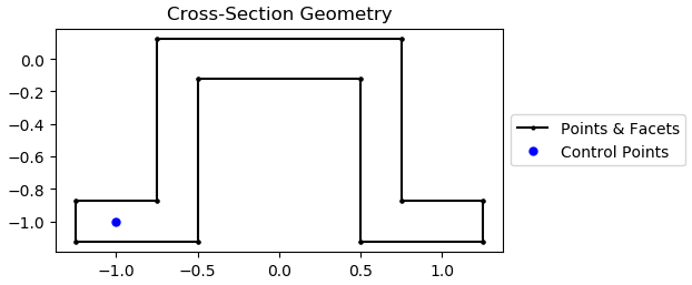
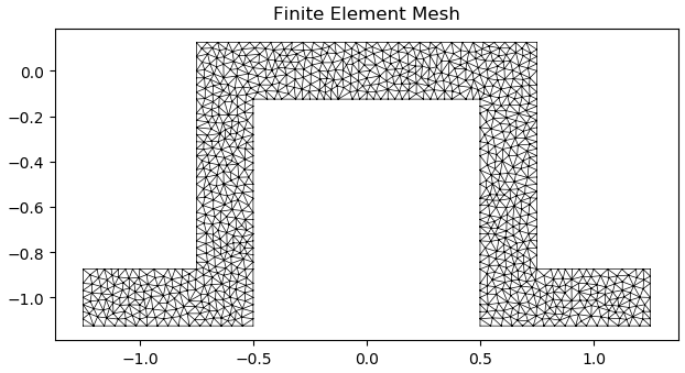
Constructs a Hat section with the top most section’s middle center at the origin (0, 0),
with four parameters defining dimensions. See Nastran documentation 1234 for
more details. Note that HAT in ASTROS is actually HAT1 in this code. Added by JohnDN90.
Parameters
DIM1 (float) – Depth (y) of HAT-section
DIM2 (float) – Thickness of HAT-section
DIM3 (float) – Width (x) of top most section
DIM4 (float) – Width (x) of bottom sections
Optional[sectionproperties.pre.pre.Material] – Material to associate with this geometry
The following example creates a HAT cross-section with a depth of 1.25 and width of 2.5, and
generates a mesh with a maximum triangular area of 0.001:
Constructs a HAT1 section with the bottom plate’s bottom center at the origin (0, 0),
with five parameters defining dimensions. See Nastran documentation 1235 for
definition of parameters. Note that in ASTROS, HAT1 is called HAT. Added by JohnDN90.
Parameters
DIM1 (float) – Width(x) of the HAT1-section
DIM2 (float) – Depth (y) of the HAT1-section
DIM3 (float) – Width (x) of hat’s top flange
DIM4 (float) – Thickness of hat stiffener
DIM5 (float) – Thicknesss of bottom plate
Optional[sectionproperties.pre.pre.Material] – Material to associate with this geometry
The following example creates a HAT1 cross-section with a depth of 2.0 and width of 4.0, and
generates a mesh with a maximum triangular area of 0.005:
Constructs a HEXA (hexagon) section with the center at the origin (0, 0), with three
parameters defining dimensions. See Nastran documentation 1234 for more details.
Added by JohnDN90.
Parameters
DIM1 (float) – Spacing between bottom right point and right most point
DIM2 (float) – Width (x) of hexagon
DIM3 (float) – Depth (y) of hexagon
Optional[sectionproperties.pre.pre.Material] – Material to associate with this geometry
The following example creates a rectangular cross-section with a depth of 1.5 and width of 2.0,
and generates a mesh with a maximum triangular area of 0.005:
Constructs Nastran’s I section with the bottom flange’s middle center at the origin
(0, 0), with six parameters defining dimensions. See Nastran documentation 1234 for definition of parameters. Added by JohnDN90.
Parameters
DIM1 (float) – Depth(y) of the I Section
DIM2 (float) – Width (x) of bottom flange
DIM3 (float) – Width (x) of top flange
DIM4 (float) – Thickness of web
DIM5 (float) – Thickness of bottom web
DIM6 (float) – Thickness of top web
Optional[sectionproperties.pre.pre.Material] – Material to associate with this geometry
The following example creates a Nastran I cross-section with a depth of 5.0, and generates a
mesh with a maximum triangular area of 0.008:
Constructs a I1 section with the web’s middle center at the origin (0, 0), with four
parameters defining dimensions. See Nastran documentation 1234 for more details.
Added by JohnDN90.
Parameters
DIM1 (float) – Twice distance from web end to flange end
DIM2 (float) – Thickness of web
DIM3 (float) – Length of web (spacing between flanges)
DIM4 (float) – Depth (y) of the I1-section
Optional[sectionproperties.pre.pre.Material] – Material to associate with this geometry
The following example creates a I1 cross-section with a depth of
5.0 and width of 1.75, and generates a mesh with a maximum triangular area of
0.02:
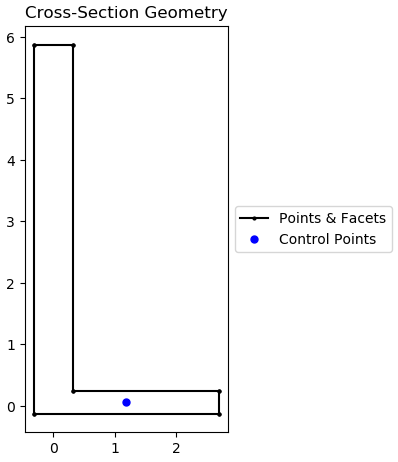
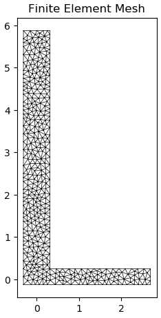
Constructs a L section with the intersection’s center at the origin (0, 0), with four
parameters defining dimensions. See Nastran documentation 123 for more details.
Added by JohnDN90.
Parameters
DIM1 (float) – Width (x) of the L-section
DIM2 (float) – Depth (y) of the L-section
DIM3 (float) – Thickness of flange (horizontal portion)
DIM4 (float) – Thickness of web (vertical portion)
Optional[sectionproperties.pre.pre.Material] – Material to associate with this geometry
The following example creates a L cross-section with a depth of 6.0 and width of 3.0, and
generates a mesh with a maximum triangular area of 0.01:
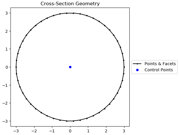
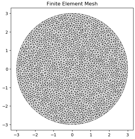
Constructs a circular rod section with the center at the origin (0, 0), with one parameter
defining dimensions. See Nastran documentation 1234 for more details. Added by
JohnDN90.
Parameters
DIM1 (float) – Radius of the circular rod section
n (int) – Number of points discretising the circle
Optional[sectionproperties.pre.pre.Material] – Material to associate with this geometry
The following example creates a circular rod with a radius of 3.0 and 50 points discretising
the boundary, and generates a mesh with a maximum triangular area of 0.01:
Constructs a T section with the top flange’s middle center at the origin (0, 0), with four
parameters defining dimensions. See Nastran documentation 12345 for more
details. Added by JohnDN90.
Parameters
DIM1 (float) – Width (x) of top flange
DIM2 (float) – Depth (y) of the T-section
DIM3 (float) – Thickness of top flange
DIM4 (float) – Thickness of web
Optional[sectionproperties.pre.pre.Material] – Material to associate with this geometry
The following example creates a T cross-section with a depth of 4.0 and width of 3.0, and
generates a mesh with a maximum triangular area of 0.001:
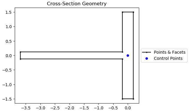
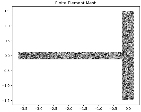
Constructs a T1 section with the right flange’s middle center at the origin (0, 0), with
four parameters defining dimensions. See Nastran documentation 1234 for more
details. Added by JohnDN90.
Parameters
DIM1 (float) – Depth (y) of T1-section
DIM2 (float) – Length (x) of web
DIM3 (float) – Thickness of right flange
DIM4 (float) – Thickness of web
Optional[sectionproperties.pre.pre.Material] – Material to associate with this geometry
The following example creates a T1 cross-section with a depth of 3.0 and width of 3.875, and
generates a mesh with a maximum triangular area of 0.001:
Constructs a T2 section with the bottom flange’s middle center at the origin (0, 0), with
four parameters defining dimensions. See Nastran documentation 1234 for more
details. Added by JohnDN90.
Parameters
DIM1 (float) – Width (x) of T2-section
DIM2 (float) – Depth (y) of T2-section
DIM3 (float) – Thickness of bottom flange
DIM4 (float) – Thickness of web
Optional[sectionproperties.pre.pre.Material] – Material to associate with this geometry
The following example creates a T2 cross-section with a depth of 4.0 and width of 3.0, and
generates a mesh with a maximum triangular area of 0.005:
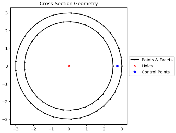
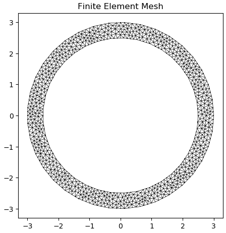
Constructs a circular tube section with the center at the origin (0, 0), with two
parameters defining dimensions. See Nastran documentation 1234 for more
details. Added by JohnDN90.
Parameters
DIM1 (float) – Outer radius of the circular tube section
DIM2 (float) – Inner radius of the circular tube section
n (int) – Number of points discretising the circle
Optional[sectionproperties.pre.pre.Material] – Material to associate with this geometry
The following example creates a circular tube cross-section with an outer radius of 3.0 and an
inner radius of 2.5, and generates a mesh with 37 points discretising the boundaries and a
maximum triangular area of 0.01:
Constructs a circular TUBE2 section with the center at the origin (0, 0), with two
parameters defining dimensions. See MSC Nastran documentation 1 for more details. Added by
JohnDN90.
Parameters
DIM1 (float) – Outer radius of the circular tube section
DIM2 (float) – Thickness of wall
n (int) – Number of points discretising the circle
Optional[sectionproperties.pre.pre.Material] – Material to associate with this geometry
The following example creates a circular TUBE2 cross-section with an outer radius of 3.0 and a
wall thickness of 0.5, and generates a mesh with 37 point discretising the boundary and a
maximum triangular area of 0.01:
Constructs a Z section with the web’s middle center at the origin (0, 0), with four
parameters defining dimensions. See Nastran documentation 1234 for more details.
Added by JohnDN90.
Parameters
DIM1 (float) – Width (x) of horizontal members
DIM2 (float) – Thickness of web
DIM3 (float) – Spacing between horizontal members (length of web)
DIM4 (float) – Depth (y) of Z-section
Optional[sectionproperties.pre.pre.Material] – Material to associate with this geometry
The following example creates a rectangular cross-section with a depth of 4.0 and width of
2.75, and generates a mesh with a maximum triangular area of 0.005:
Stores the finite element geometry, mesh and material information and provides methods to
compute the cross-section properties. The element type used in this program is the six-noded
quadratic triangular element.
The constructor extracts information from the provided mesh object and creates and stores the
corresponding Tri6 finite element objects.
Parameters
geometry (Geometry) – Cross-section geometry object used to generate the mesh
time_info (bool) – If set to True, a detailed description of the computation and the time
cost is printed to the terminal for every computation performed.
The following example creates a Section
object of a 100D x 50W rectangle using a mesh size of 5:
Assembles stiffness matrices to be used for the computation of warping
properties and the torsion load vector (f_torsion). A Lagrangian multiplier
(k_lg) stiffness matrix is returned. The stiffness matrix are assembled using
the sparse COO format and returned in the sparse CSC format.
Returns
Lagrangian multiplier stiffness matrix and torsion load
vector (k_lg, f_torsion)
Calculates and returns the properties required for a frame analysis. The properties are
also stored in the SectionProperties
object contained in the section_props class variable.
Parameters
solver_type (string) – Solver used for solving systems of linear equations, either
using the ‘direct’ method or ‘cgs’ iterative method
Returns
Cross-section properties to be used for a frame analysis (area, ixx, iyy, ixy, j,
phi)
Return type
tuple(float, float, float, float, float, float)
The following section properties are calculated:
Cross-sectional area (area)
Second moments of area about the centroidal axis (ixx, iyy, ixy)
Torsion constant (j)
Principal axis angle (phi)
If materials are specified for the cross-section, the area, second moments of area and
torsion constant are elastic modulus weighted.
The following example demonstrates the use of this method:
Calculates the geometric properties of the cross-section and stores them in the
SectionProperties object contained in
the section_props class variable.
The following geometric section properties are calculated:
Cross-sectional area
Cross-sectional perimeter
Cross-sectional mass
Area weighted material properties, composite only \(E_{eff}\), \(G_{eff}\), \({nu}_{eff}\)
Modulus weighted area (axial rigidity)
First moments of area
Second moments of area about the global axis
Second moments of area about the centroidal axis
Elastic centroid
Centroidal section moduli
Radii of gyration
Principal axis properties
If materials are specified for the cross-section, the moments of area and section moduli
are elastic modulus weighted.
The following example demonstrates the use of this method:
Calculates the plastic properties of the cross-section and stores them in the
SectionProperties object contained in
the section_props class variable.
Parameters
verbose (bool) – If set to True, the number of iterations required for each plastic
axis is printed to the terminal.
The following warping section properties are calculated:
Plastic centroid for bending about the centroidal and principal axes
Plastic section moduli for bending about the centroidal and principal axes
Shape factors for bending about the centroidal and principal axes
If materials are specified for the cross-section, the plastic section moduli are displayed
as plastic moments (i.e \(M_p = f_y S\)) and the shape factors are not calculated.
Note that the geometric properties must be calculated before the plastic properties are
calculated:
Note that a geometric analysis must be performed prior to performing a stress
analysis. Further, if the shear force or torsion is non-zero a warping analysis
must also be performed:
Calculates all the warping properties of the cross-section and stores them in the
SectionProperties object contained in
the section_props class variable.
Parameters
solver_type (string) – Solver used for solving systems of linear equations, either
using the ‘direct’ method or ‘cgs’ iterative method
The following warping section properties are calculated:
Torsion constant
Shear centre
Shear area
Warping constant
Monosymmetry constant
If materials are specified, the values calculated for the torsion constant, warping
constant and shear area are elastic modulus weighted.
Note that the geometric properties must be calculated prior to the calculation of the
warping properties:
Monosymmetry constant for bending about both global axes (beta_x_plus,
beta_x_minus, beta_y_plus, beta_y_minus). The plus value relates to the top flange
in compression and the minus value relates to the bottom flange in compression.
Monosymmetry constant for bending about both principal axes (beta_11_plus,
beta_11_minus, beta_22_plus, beta_22_minus). The plus value relates to the top
flange in compression and the minus value relates to the bottom flange in
compression.
Calculates the stress at a point within an element for given design actions
and returns (sigma_zz, tau_xz, tau_yz)
Parameters
pt (list[float, float]) – The point. A list of the x and y coordinate
N (float) – Axial force
Vx (float) – Shear force acting in the x-direction
Vy (float) – Shear force acting in the y-direction
Mxx (float) – Bending moment about the centroidal xx-axis
Myy (float) – Bending moment about the centroidal yy-axis
M11 (float) – Bending moment about the centroidal 11-axis
M22 (float) – Bending moment about the centroidal 22-axis
Mzz (float) – Torsion moment about the centroidal zz-axis
agg_function (function, optional) – A function that aggregates the stresses if the point is shared by several elements.
If the point, pt, is shared by several elements (e.g. if it is a node or on an edge), the stress
(sigma_zz, tau_xz, tau_yz) are retrieved from each element and combined according to this function.
By default, numpy.average is used.
Returns
Resultant normal and shear stresses list[(sigma_zz, tau_xz, tau_yz)]. If a point it not in the
section then None is returned.
Calculates the stress at a set of points within an element for given design actions
and returns (sigma_zz, tau_xz, tau_yz)
Parameters
pts (list[list[float, float]]) – The points. A list of several x and y coordinates
N (float) – Axial force
Vx (float) – Shear force acting in the x-direction
Vy (float) – Shear force acting in the y-direction
Mxx (float) – Bending moment about the centroidal xx-axis
Myy (float) – Bending moment about the centroidal yy-axis
M11 (float) – Bending moment about the centroidal 11-axis
M22 (float) – Bending moment about the centroidal 22-axis
Mzz (float) – Torsion moment about the centroidal zz-axis
agg_function (function, optional) – A function that aggregates the stresses if the point is shared by several elements.
If the point, pt, is shared by several elements (e.g. if it is a node or on an edge), the stress
(sigma_zz, tau_xz, tau_yz) are retrieved from each element and combined according to this function.
By default, numpy.average is used.
Returns
Resultant normal and shear stresses list[(sigma_zz, tau_xz, tau_yz)]. If a point it not in the
section then None is returned for that element in the list.
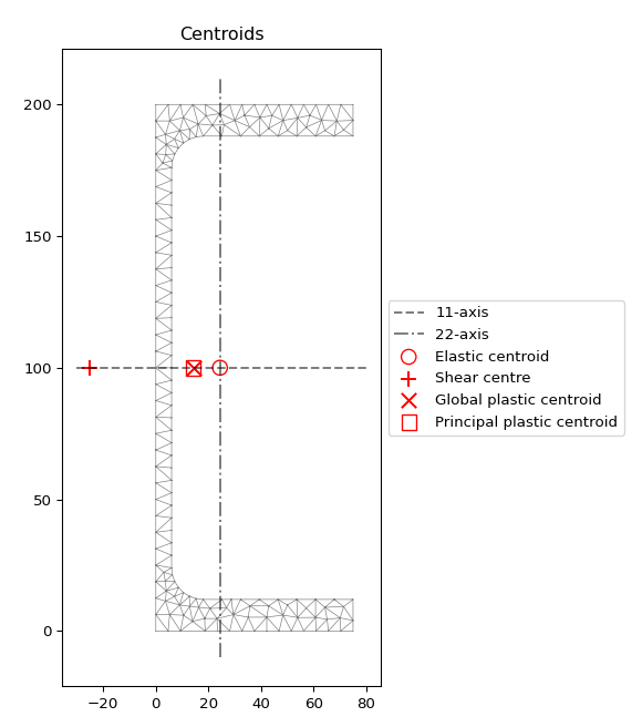
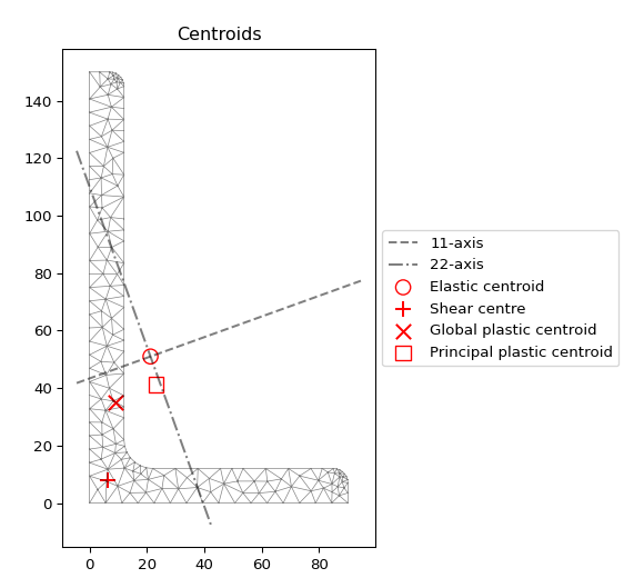
Plots the elastic centroid, the shear centre, the plastic centroids and the principal
axis, if they have been calculated, on top of the finite element mesh.
Calculates the location of the plastic centroid with respect to the centroidal and
principal bending axes, the plastic section moduli and shape factors and stores the results
to the supplied Section object.
Parameters
section (Section) – Cross section object that uses the same geometry and materials
specified in the class constructor
verbose (bool) – If set to True, the number of iterations required for each plastic
axis is printed to the terminal.
Given a distance d from the centroid to an axis (defined by unit vector u), creates
a mesh including the new and axis and calculates the force equilibrium. The resultant
force, as a ratio of the total force, is returned.
Parameters
d (float) – Distance from the centroid to current axis
u (numpy.ndarray) – Unit vector defining the direction of the axis
u_p (numpy.ndarray) – Unit vector perpendicular to the direction of the axis
verbose (bool) – If set to True, the number of iterations required for each plastic
axis is printed to the terminal.
An algorithm used for solving for the location of the plastic centroid. The algorithm
searches for the location of the axis, defined by unit vector u and within the section
depth, that satisfies force equilibrium.
Parameters
u (numpy.ndarray) – Unit vector defining the direction of the axis
dlim (list[float, float]) – List [dmax, dmin] containing the distances from the centroid to the extreme
fibres perpendicular to the axis
axis (int) – The current axis direction: 1 (e.g. x or 11) or 2 (e.g. y or 22)
verbose (bool) – If set to True, the number of iterations required for each plastic
axis is printed to the terminal.
Returns
The distance to the plastic centroid axis d, the result object r, the force in
the top of the section f_top and the location of the centroids of the top and bottom
areas c_top and c_bottom
Class for post-processing finite element stress results.
A StressPost object is created when a stress analysis is carried out and is returned as an
object to allow post-processing of the results. The StressPost object creates a deep copy of
the MaterialGroups within the cross-section to allow the calculation of stresses for each
material. Methods for post-processing the calculated stresses are provided.
Parameters
section (Section) – Cross section object for stress calculation
Variables
section (Section) – Cross section object for stress calculation
material_groups (list[MaterialGroup]) – A deep copy of the section material groups to allow a new stress
analysis
Returns the stresses within each material belonging to the current
StressPost object.
Returns
A list of dictionaries containing the cross-section stresses for each material.
Return type
list[dict]
A dictionary is returned for each material in the cross-section, containing the following
keys and values:
‘Material’: Material name
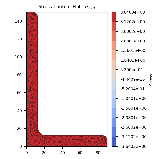
‘sig_zz_n’: Normal stress \(\sigma_{zz,N}\) resulting from the axial load \(N\)
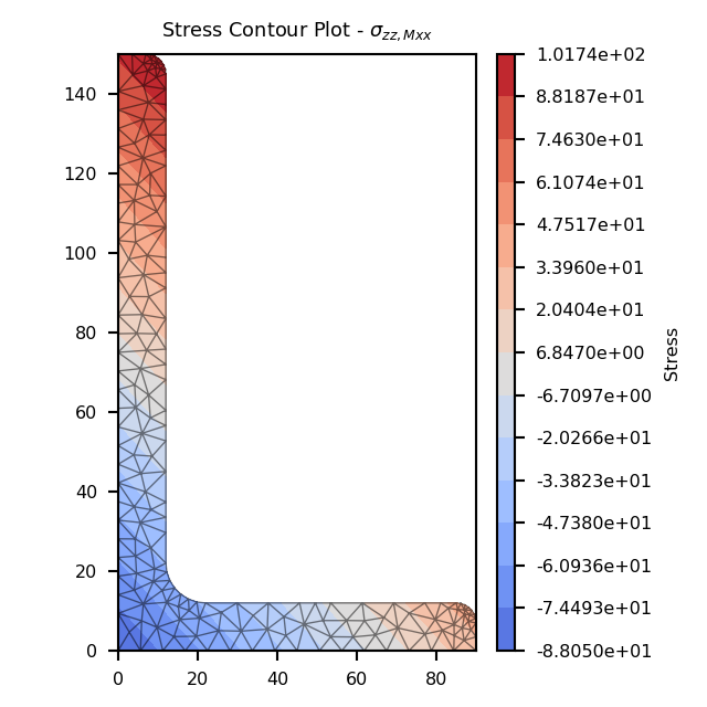
‘sig_zz_mxx’: Normal stress \(\sigma_{zz,Mxx}\) resulting from the bending moment
\(M_{xx}\)
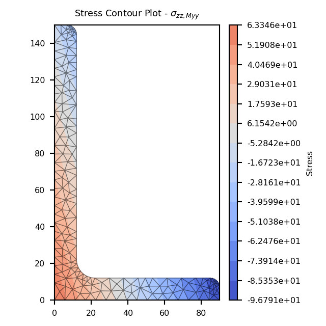
‘sig_zz_myy’: Normal stress \(\sigma_{zz,Myy}\) resulting from the bending moment
\(M_{yy}\)
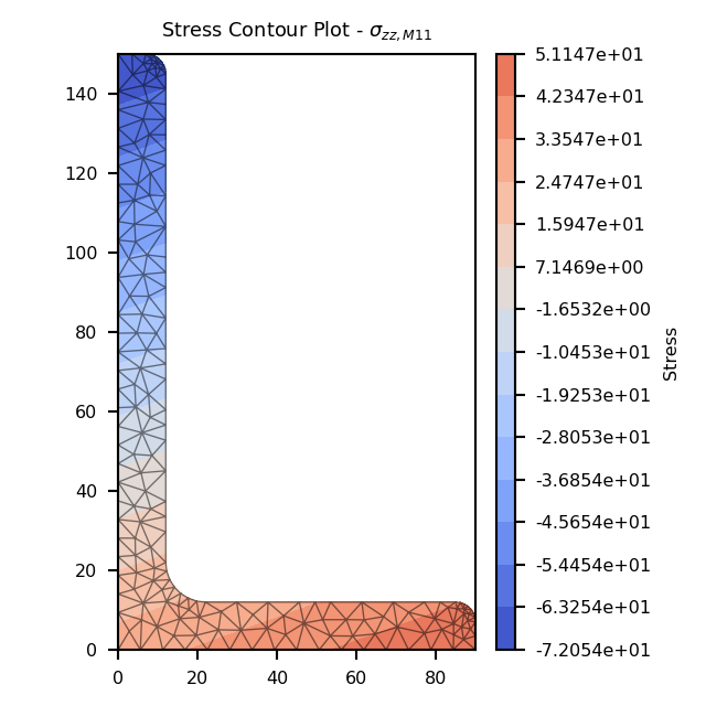
‘sig_zz_m11’: Normal stress \(\sigma_{zz,M11}\) resulting from the bending moment
\(M_{11}\)
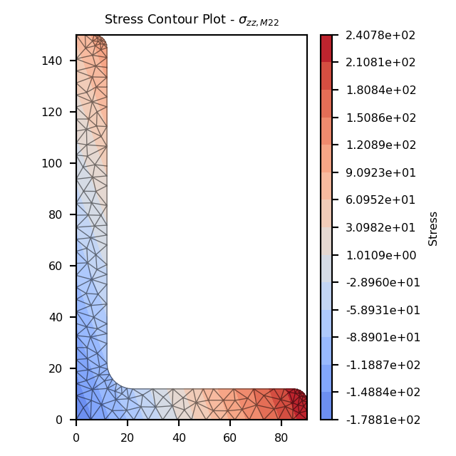
‘sig_zz_m22’: Normal stress \(\sigma_{zz,M22}\) resulting from the bending moment
\(M_{22}\)
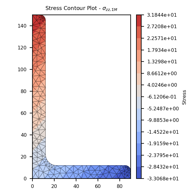
‘sig_zz_m’: Normal stress \(\sigma_{zz,\Sigma M}\) resulting from all bending
moments
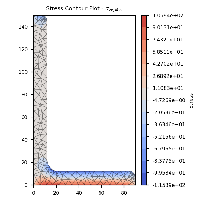
‘sig_zx_mzz’: x-component of the shear stress \(\sigma_{zx,Mzz}\) resulting from
the torsion moment
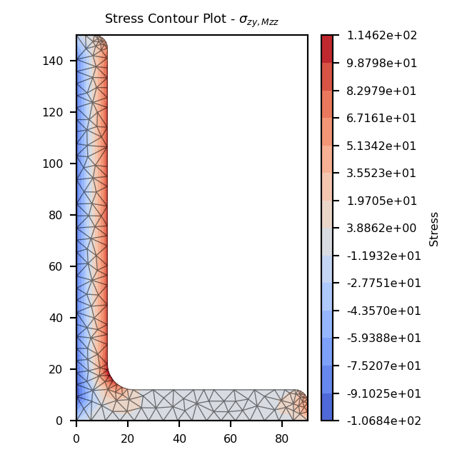
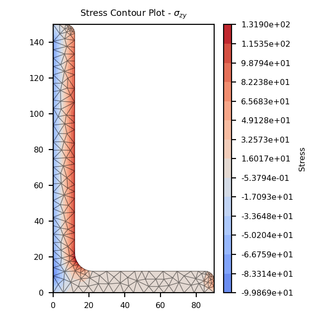
‘sig_zy_mzz’: y-component of the shear stress \(\sigma_{zy,Mzz}\) resulting from
the torsion moment
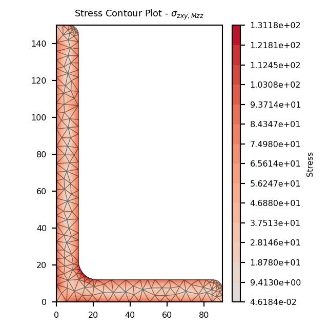
‘sig_zxy_mzz’: Resultant shear stress \(\sigma_{zxy,Mzz}\) resulting from the
torsion moment
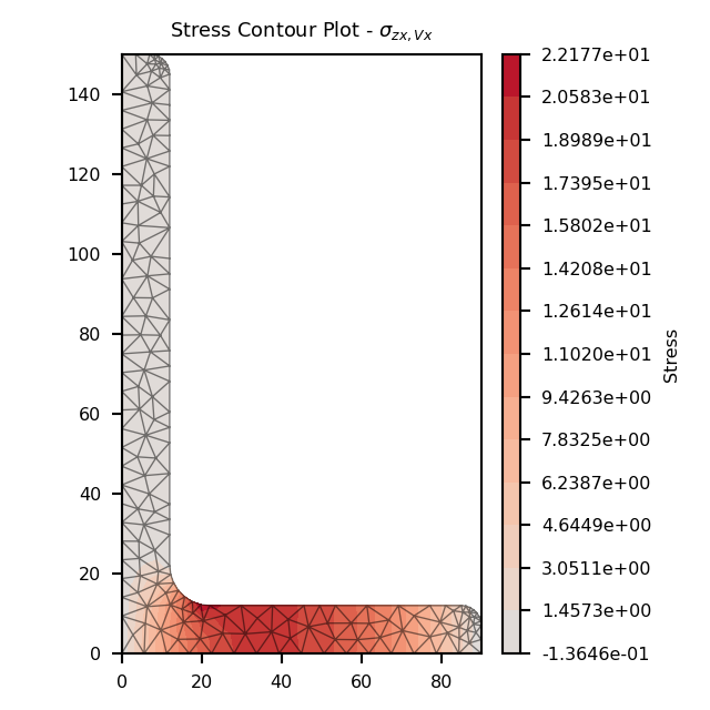
‘sig_zx_vx’: x-component of the shear stress \(\sigma_{zx,Vx}\) resulting from
the shear force \(V_{x}\)
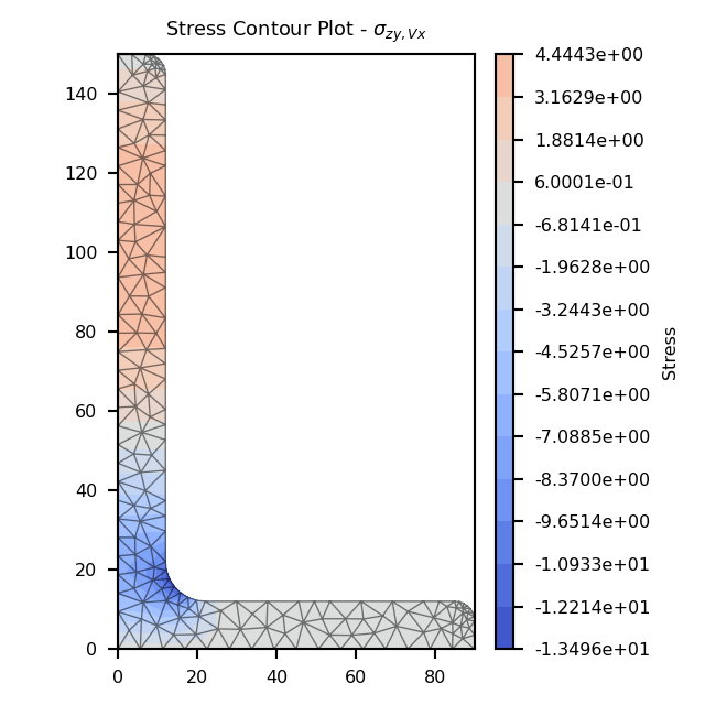
‘sig_zy_vx’: y-component of the shear stress \(\sigma_{zy,Vx}\) resulting from
the shear force \(V_{x}\)
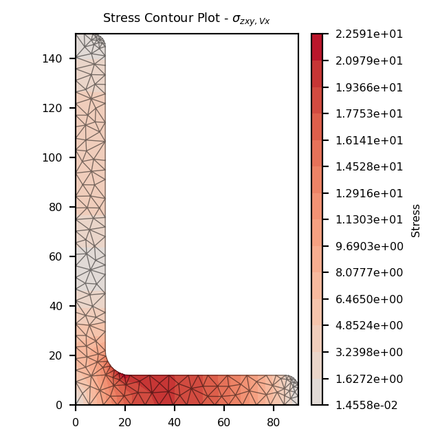
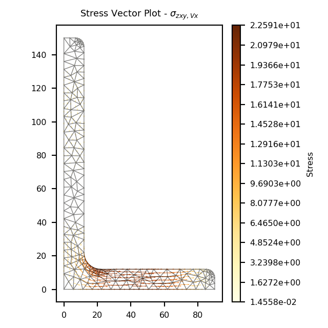
‘sig_zxy_vx’: Resultant shear stress \(\sigma_{zxy,Vx}\) resulting from the shear
force \(V_{x}\)
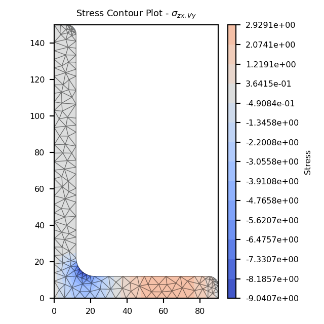
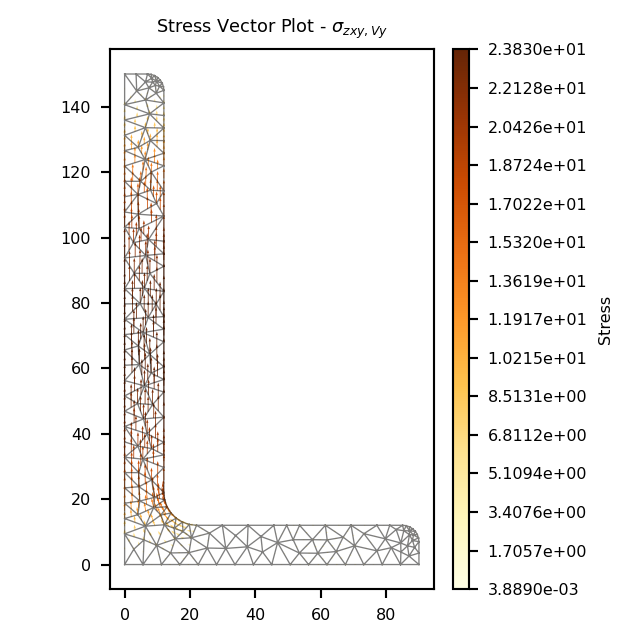
‘sig_zx_vy’: x-component of the shear stress \(\sigma_{zx,Vy}\) resulting from
the shear force \(V_{y}\)
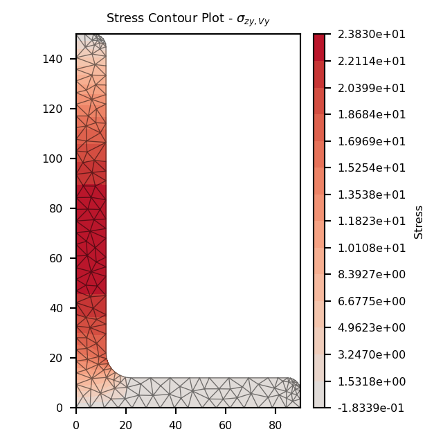
‘sig_zy_vy’: y-component of the shear stress \(\sigma_{zy,Vy}\) resulting from
the shear force \(V_{y}\)
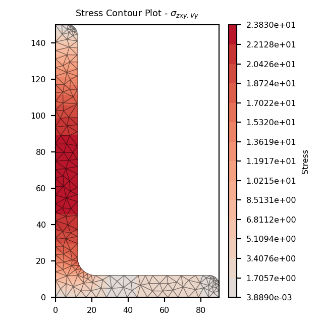
‘sig_zxy_vy’: Resultant shear stress \(\sigma_{zxy,Vy}\) resulting from the shear
force \(V_{y}\)
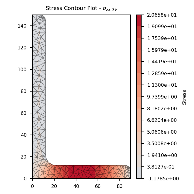
‘sig_zx_v’: x-component of the shear stress \(\sigma_{zx,\Sigma V}\) resulting
from all shear forces
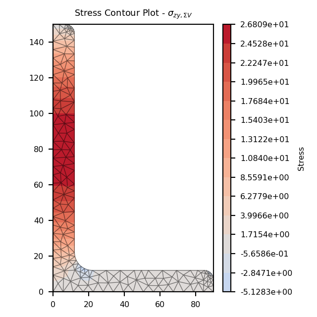
‘sig_zy_v’: y-component of the shear stress \(\sigma_{zy,\Sigma V}\) resulting
from all shear forces
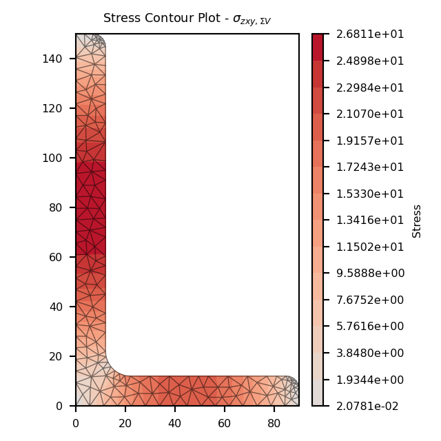
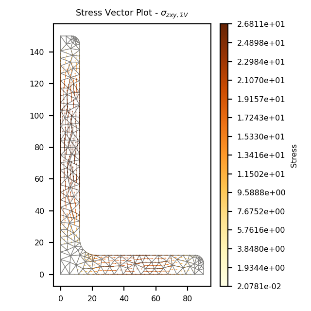
‘sig_zxy_v’: Resultant shear stress \(\sigma_{zxy,\Sigma V}\) resulting from all
shear forces
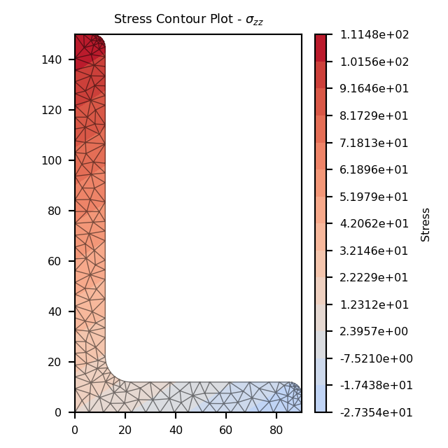
‘sig_zz’: Combined normal stress \(\sigma_{zz}\) resulting from all actions
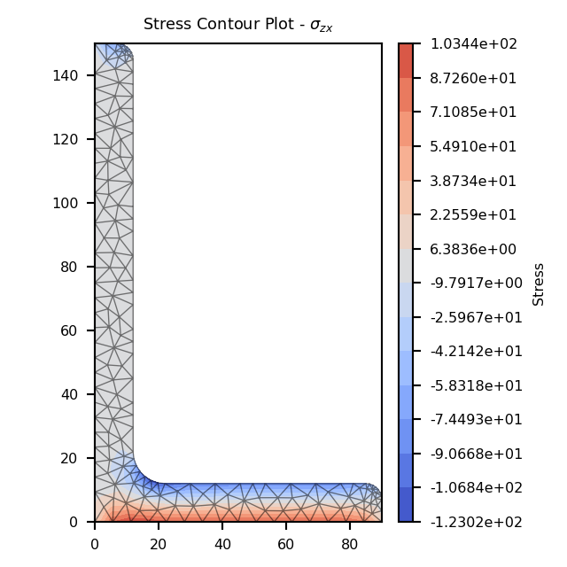
‘sig_zx’: x-component of the shear stress \(\sigma_{zx}\) resulting from all
actions
‘sig_zy’: y-component of the shear stress \(\sigma_{zy}\) resulting from all
actions
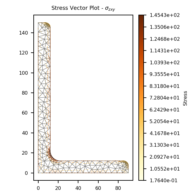
‘sig_zxy’: Resultant shear stress \(\sigma_{zxy}\) resulting from all actions
‘sig_1’: Major principal stress \(\sigma_{1}\) resulting from all actions
‘sig_3’: Minor principal stress \(\sigma_{3}\) resulting from all actions
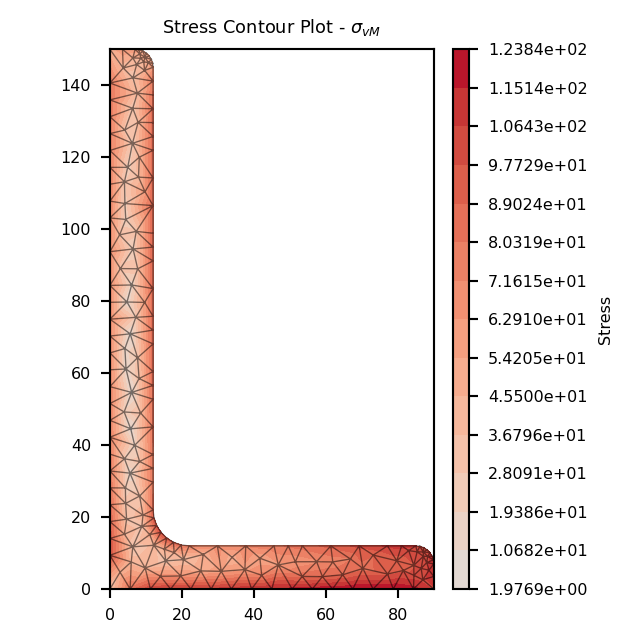
‘sig_vm’: von Mises stress \(\sigma_{vM}\) resulting from all actions
The following example returns stresses for each material within a composite section, note
that a result is generated for each node in the mesh for all materials irrespective of
whether the materials exists at that point or not.
The following example plots the normal stress within a 150x90x12 UA section resulting from
a bending moment about the x-axis of 5 kN.m, a bending moment about the y-axis of 2 kN.m
and a bending moment of 3 kN.m about the 11-axis:
Produces a contour plot of the x-component of the shear stress
\(\sigma_{zx,\Sigma V}\) resulting from the sum of the applied shear forces
\(V_{x} + V_{y}\).
Parameters
title (string) – Plot title
cmap (string) – Matplotlib color map.
normalize (bool) – If set to true, the CenteredNorm is used to scale the colormap.
If set to false, the default linear scaling is used.
The following example plots the x-component of the shear stress within a 150x90x12 UA
section resulting from a shear force of 15 kN in the x-direction and 30 kN in the
y-direction:
The following example plots a contour of the resultant shear stress within a 150x90x12 UA
section resulting from a shear force of 15 kN in the x-direction and 30 kN in the
y-direction:
Produces a contour plot of the y-component of the shear stress
\(\sigma_{zy,\Sigma V}\) resulting from the sum of the applied shear forces
\(V_{x} + V_{y}\).
Parameters
title (string) – Plot title
cmap (string) – Matplotlib color map.
normalize (bool) – If set to true, the CenteredNorm is used to scale the colormap.
If set to false, the default linear scaling is used.
The following example plots the y-component of the shear stress within a 150x90x12 UA
section resulting from a shear force of 15 kN in the x-direction and 30 kN in the
y-direction:
The following example plots the x-component of the shear stress within a 150x90x12 UA
section resulting from a shear force in the x-direction of 15 kN:
The following example plots a contour of the resultant shear stress within a 150x90x12 UA
section resulting from a shear force in the x-direction of 15 kN:
The following example plots the y-component of the shear stress within a 150x90x12 UA
section resulting from a shear force in the x-direction of 15 kN:
The following example plots the x-component of the shear stress within a 150x90x12 UA
section resulting from a shear force in the y-direction of 30 kN:
The following example plots a contour of the resultant shear stress within a 150x90x12 UA
section resulting from a shear force in the y-direction of 30 kN:
The following example plots the y-component of the shear stress within a 150x90x12 UA
section resulting from a shear force in the y-direction of 30 kN:
The following example plots the x-component of the shear stress within a 150x90x12 UA
section resulting from a torsion moment of 1 kN.m and a shear force of 30 kN in the
y-direction:
The following example plots a contour of the resultant shear stress within a 150x90x12 UA
section resulting from a torsion moment of 1 kN.m and a shear force of 30 kN in the
y-direction:
The following example plots the y-component of the shear stress within a 150x90x12 UA
section resulting from a torsion moment of 1 kN.m and a shear force of 30 kN in the
y-direction:
The following example plots the normal stress within a 150x90x12 UA section resulting from
an axial force of 100 kN, a bending moment about the x-axis of 5 kN.m and a bending moment
about the y-axis of 2 kN.m:
The following example generates a vector plot of the shear stress within a 150x90x12 UA
section resulting from a shear force of 15 kN in the x-direction and 30 kN in the
y-direction:
The following example generates a vector plot of the shear stress within a 150x90x12 UA
section resulting from a shear force in the x-direction of 15 kN:
The following example generates a vector plot of the shear stress within a 150x90x12 UA
section resulting from a shear force in the y-direction of 30 kN:
The following example generates a vector plot of the shear stress within a 150x90x12 UA
section resulting from a torsion moment of 1 kN.m and a shear force of 30 kN in the
y-direction:
Class for storing elements of different materials.
A MaterialGroup object contains the finite element objects for a specified material. The
stress_result variable provides storage for stresses related each material.
Parameters
material (Material) – Material object for the current MaterialGroup
num_nods (int) – Number of nodes for the entire cross-section
Variables
material (Material) – Material object for the current MaterialGroup
stress_result (StressResult) – A StressResult object for saving the stresses of the current material
elements (list[Tri6]) – A list of finite element objects that are of the current material type
el_ids (list[int]) – A list of the element IDs of the elements that are of the current material type
Class for a six noded quadratic triangular element.
Provides methods for the calculation of section properties based on the finite element method.
Parameters
el_id (int) – Unique element id
coords (numpy.ndarray) – A 2 x 6 array of the coordinates of the tri-6 nodes. The first three columns
relate to the vertices of the triangle and the last three columns correspond to the
mid-nodes.
node_ids (list[int]) – A list of the global node ids for the current element
material (Material) – Material object for the current finite element.
Variables
el_id (int) – Unique element id
coords (numpy.ndarray) – A 2 x 6 array of the coordinates of the tri-6 nodes. The first three columns
relate to the vertices of the triangle and the last three columns correspond to the
mid-nodes.
node_ids (list[int]) – A list of the global node ids for the current element
material (Material) – Material of the current finite element.
Computes shape functions, shape function derivatives and the determinant of the Jacobian
matrix for a tri 6 element at a given Gauss point.
Parameters
coords (numpy.ndarray) – Global coordinates of the quadratic triangle vertices [2 x 6]
gauss_point (numpy.ndarray) – Gaussian weight and isoparametric location of the Gauss point
Returns
The value of the shape functions N(i) at the given Gauss point [1 x 6], the
derivative of the shape functions in the j-th global direction B(i,j) [2 x 6] and the
determinant of the Jacobian matrix j
Executes code required to set up a matplotlib figure.
Parameters
ax (matplotlib.axes.Axes) – Axes object on which to plot
pause (bool) – If set to true, the figure pauses the script until the window is closed. If
set to false, the script continues immediately after the window is rendered.
title (string) – Plot title
filename (string) – Pass a non-empty string or path to save the image as. If this option is
used, the figure is closed after the file is saved.
render (bool) – If set to False, the image is not displayed. This may be useful if the
figure or axes will be embedded or further edited before being displayed.
axis_index (Union[None, int, Tuple(int)]) – If more than 1 axes is created by subplot, then this is the axis to plot on.
This may be a tuple if a 2D array of plots is returned. The default value of None will
select the top left plot.