Advanced Geometry Creation

The below tutorial was created to demonstrate the creation of valid geometries for section analysis by combining multiple shapes.

Some key points to remember:

1. Geometries of two different materials should not overlap (can create unpredictable results)

2. If two geometries of the same materials are overlapping, then you should perform a union on the two sections

3. Two different section geometries that share a common edge (facet) should also share the same nodes (do not leave “floating” nodes along common edges)

These are general points to remember for any finite element analysis.

Note

sectionproperties will not prevent the creation of these ambiguous sections. The flexibility of the new pre-processing engine (shapely) allows for a wide variety of intermediate modelling steps but the user must ensure that the final model is one that is appropriate for analysis.

Creating Merged Sections

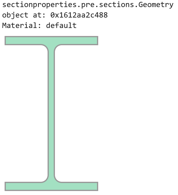
For this example, we will create a custom section out of two similar “I” sections:

import sectionproperties.pre.library.steel_sections as steel_sections
import sectionproperties.analysis.section as cross_section

i_sec1 = steel_sections.i_section(d=250, b=150, t_f=13, t_w=10, r=12, n_r=12)
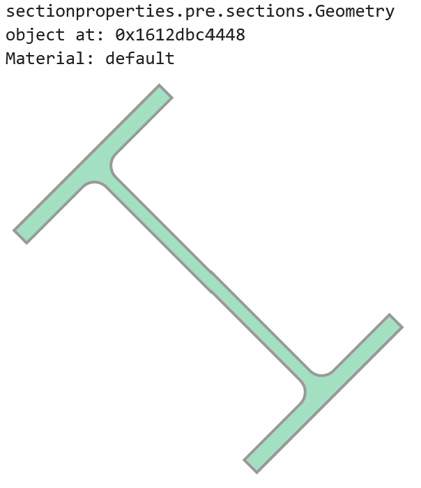
i_sec2 = i_sec1.rotate_section(45)

Assign a unique material to each geometry:

from sectionproperties.pre.pre import Material

mat1 = Material("Material_1", 200e3, 0.3, 100, 400, "red")
mat2 = Material("Material_2", 150e3, 0.2, 100, 200, "blue")  # Just some differing properties

i_sec1.material = mat1
i_sec2.material = mat2

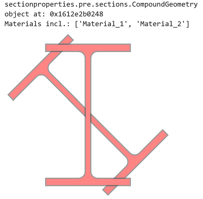
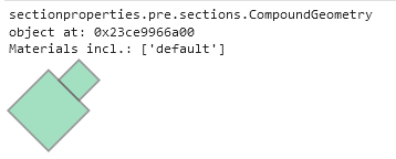
Now, we can use the + operator to naively combine these two sections into a CompoundGeometry. Note, the two different materials:

i_sec1 + i_sec2

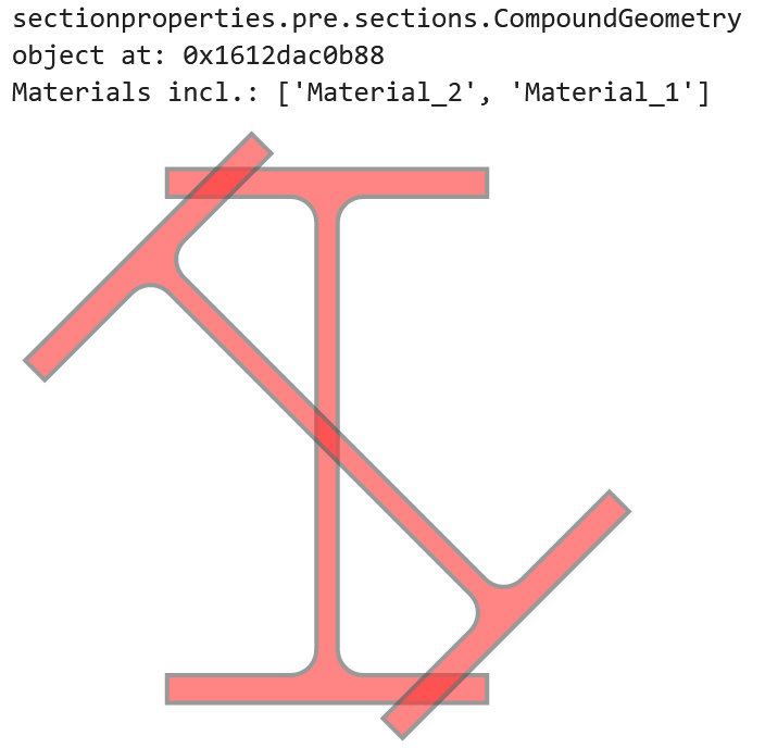
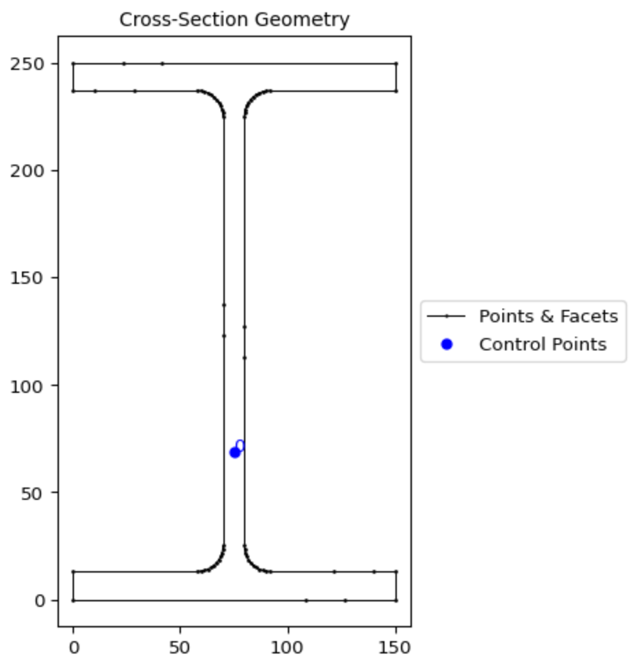
When we plot the geometry, we will see that even though we have two materials, we only have one control point for both geometries:

(i_sec1 + i_sec2).plot_geometry()

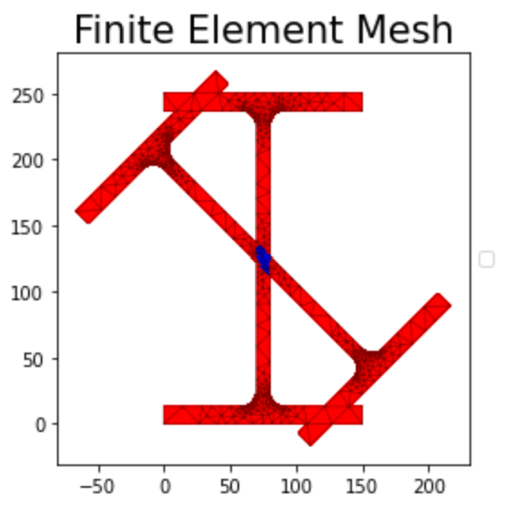
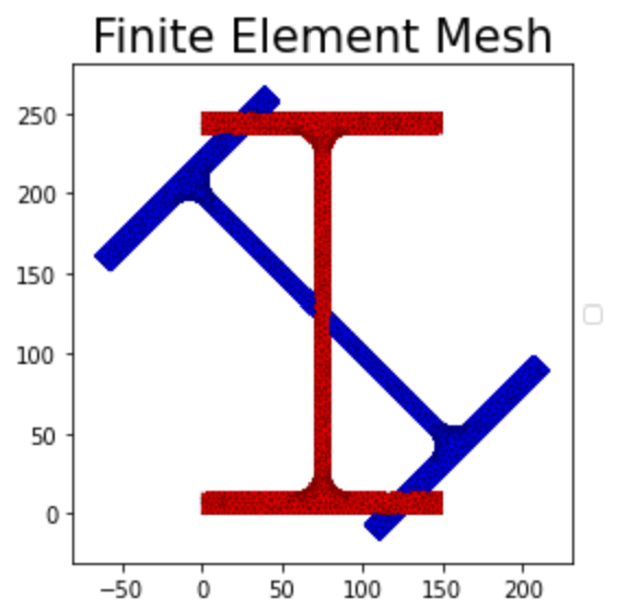
If we went a few steps further by creating a mesh and then plotting that mesh as part of an analysis section, we would see the unpredictable result of the mesh:

cross_section.Section((i_sec1 + i_sec2).create_mesh([10])).plot_mesh()

Preventing Ambiguity

To prevent ambiguity between geometries and their analytical regions, there are a few options we can take. We can perform a simple union operation but that will lose the material information for one of our sections: whichever section comes first in the operation will have it’s information preserved. In this example, we will use | (union) with i_sec2 taking precedence by being the first object in the operation:

i_sec2 | i_sec1

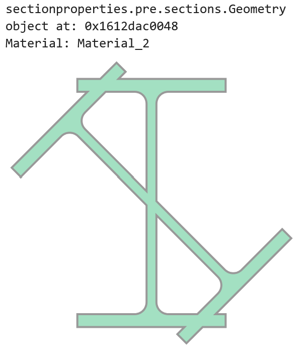
However, this is unsatisfactory as a solution. We want this section to more aptly represent a real section that might be created by cutting and welding two sections together.

Lets say we want the upright “I” section to be our main section and the diagonal section will be added on to it.

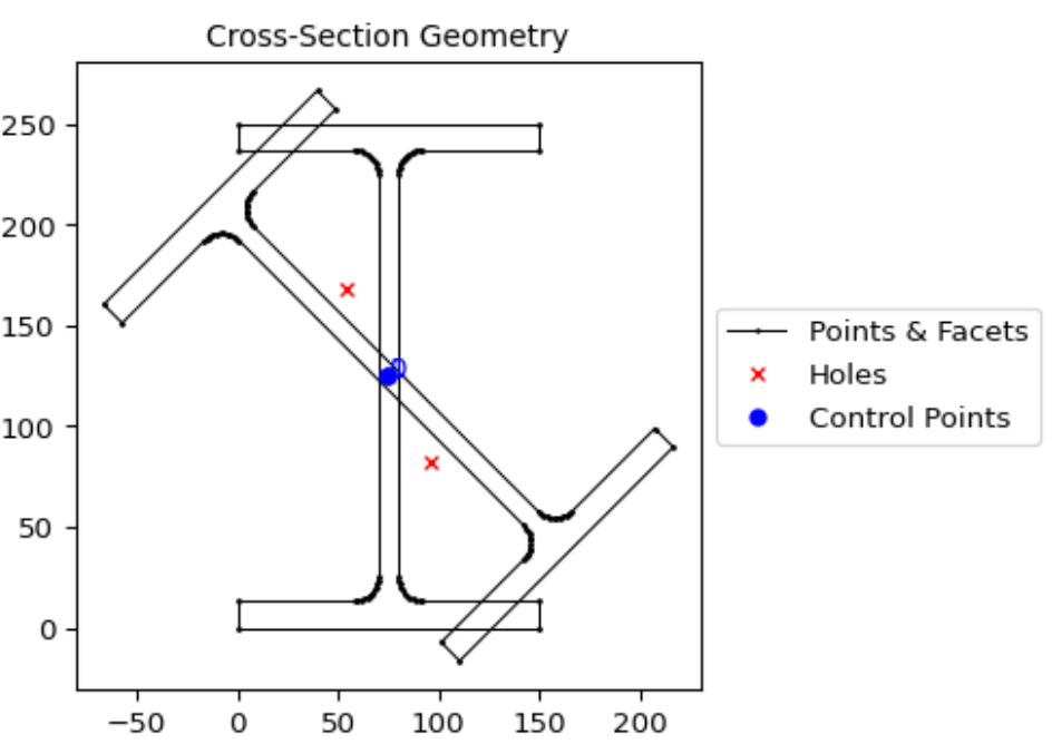
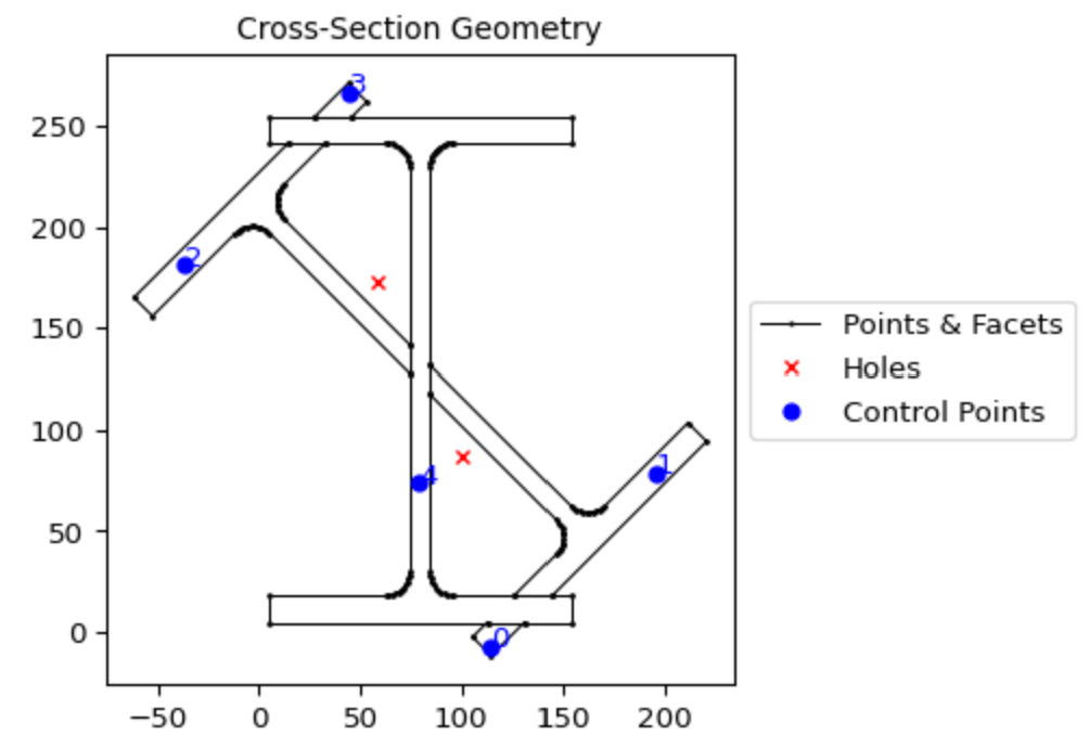
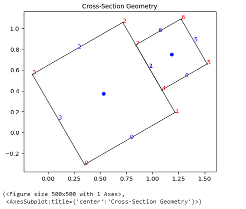
It is sometimes possible to do this in a quick operation, one which does not create nodes in common at the intersection points. Here, we will simply “slice” i_sec2 with i_sec1 and add it to i_sec1. This will create “floating nodes” along the common edges of i_sec2 and i_sec1 because the nodes are not a part of i_sec1:

(i_sec2 - i_sec1) + i_sec1

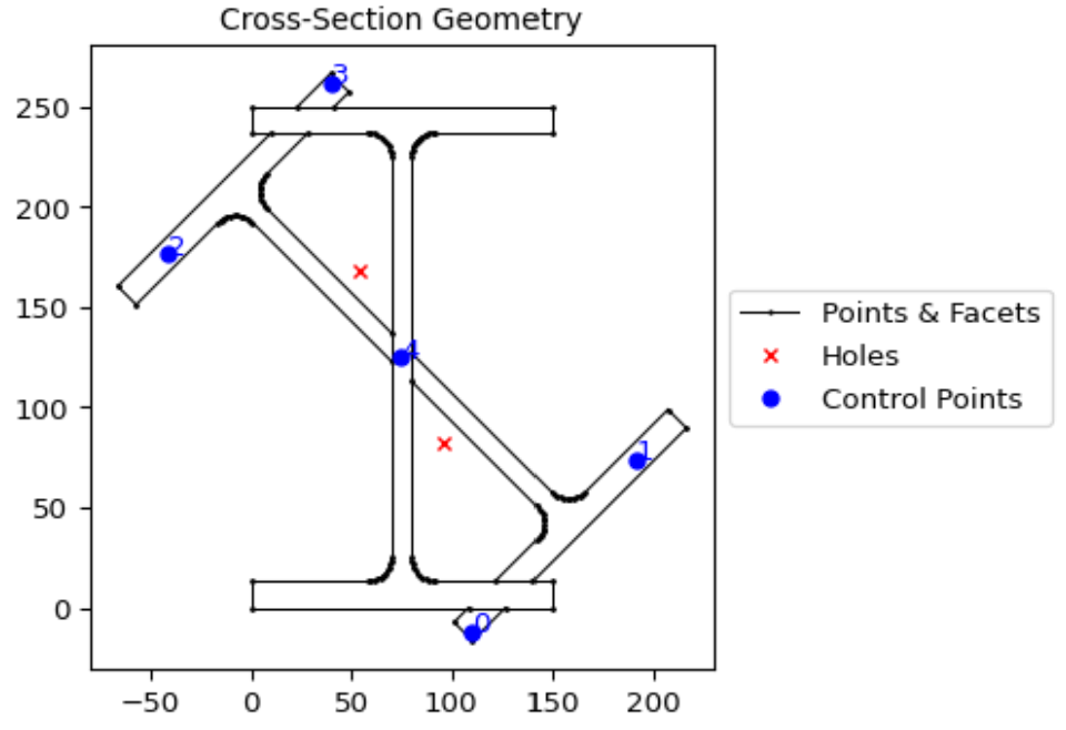
Sometimes, we can get away with this as in this example. We can see in the plot that there are five distinct regions indicated with five control points.

When we are “unlucky”, sometimes gaps can be created (due to floating point errors) where the two sections meet and a proper hole might not be detected, resulting in an incorrect section.

Creating Nodes in Common

It is best practice to first create nodes in common on both sections and then combine them. For this, an extra step is required:

cut_2_from_1 = (i_sec1 - i_sec2)  # locates intersection nodes
sec_1_nodes_added = cut_2_from_1 | i_sec1

# This can also be done in one line
sec_1_nodes_added = (i_sec1 - i_sec2) | i_sec1

Now, when we use .plot_geometry(), we can see the additional nodes added to “section 1”:

sec_1_nodes_added.plot_geometry()

The additional nodes from the cut portion are now merged as part of the “section 1” geometry.

At this point, we can use our “section 1 with additional nodes” to create our complete geometry:

analysis_geom = (i_sec2 - i_sec1) + sec_1_nodes_added
analysis_geom.plot_geometry()

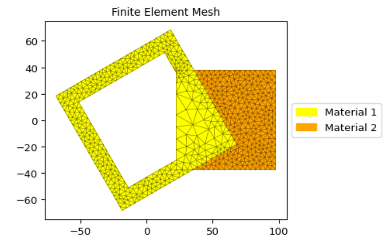
And when we create our mesh and analysis section:

analysis_geom.create_mesh([10])
analysis_sec = cross_section.Section(analysis_geom)
analysis_sec.plot_mesh()

We can see that the mesh represents how we expect the section to be.

Another example

Here, we will simply combine two squares with the default material:

import sectionproperties.pre.library.primitive_sections as primitive_sections
from sectionproperties.analysis.section import Section

s1 = primitive_sections.rectangular_section(1,1)
s2 = primitive_sections.rectangular_section(0.5,0.5).shift_section(1,0.25)
geometry = s1 + s2
geometry

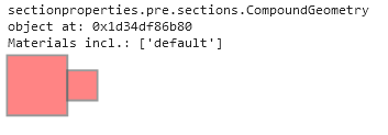
From the shapely vector representation, we can see that the squares are shaded red. This indicates an “invalid” geometry from shapely’s perspective because there are two polygons that share an edge. For this geometry, the intention is to have two squares that are connected on one side and so the red shading provided by the shapely representation tells us that we are getting what we expect.

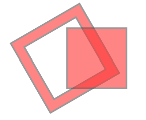
Now, say this is not our final geometry and we actually want to have it rotated by 30 degrees:

geometry = geometry.rotate_section(30)

Here, we can see that the shapely representation is now showing as green indicating a “valid” shapely geometry. Even though it is now valid for shapely, because it is green we know that these two polygons no longer share an edge because there is a miniscule separation between them as a result of a floating point error.

When we try to mesh this geometry, we will actually cause a crash with triangle, the meshing tool used behind-the-scenes by sectionproperties:

geometry.create_mesh(mesh_sizes=[0.2, 0.1]) # This may crash the kernel

The crash occurs because the distance between the two polygons is so small, even though they are separated and the space between them will not be meshed. The same crash would occur if the polygons were overlapping by this same small distance.

If we plot the geometry, you can see that each of the two squares has only four nodes and four facets and their relationship is only incidental. If their edges happen to perfectly align, they will be considered as one continuous section. If their edges do not perfectly align, they will be considered as discontinuous.

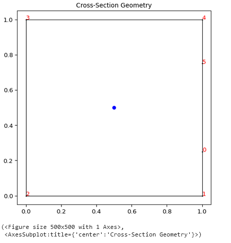
To remedy this, take the same approach as in the preceding example by creating intermediate nodes where the two polygons intersect by using set operations. If we subtract s2 from s1 then we will have the larger square with intermediate nodes created:

(s1 - s2).plot_geometry(labels=['points'])

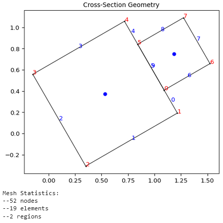
Now, if we build the compound geometry up from this larger square with the intermediate points, then our section will work.:

geometry_fixed = (s1 - s2) + s2
geometry_fixed_rotated = geometry_fixed.rotate_section(angle=30)
geometry_rot.create_mesh(mesh_sizes=[0.2, 0.1])
geometry_rot.plot_geometry(labels=["points", "facets"])
section = Section(geometry_rot)
section.display_mesh_info()

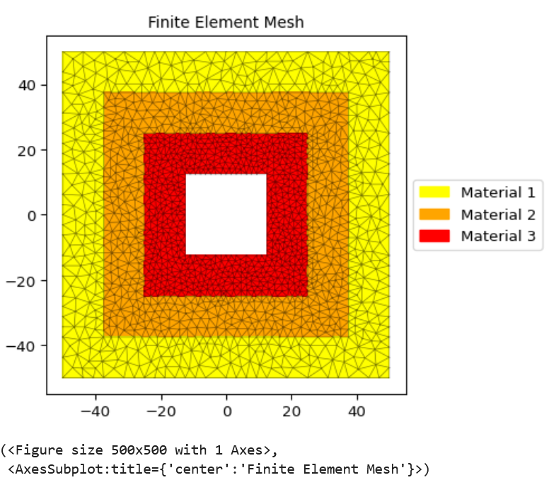
Another example (but with nested geometries)

This example demonstrates creating nested geometries using two different approaches. These approaches reflect the differences between how shapely (geometry pre-processor) “perceives” geometry and how Triangle (meshing tool) “perceives” geometry and how the modeller might adapt their input style depending on the situation.

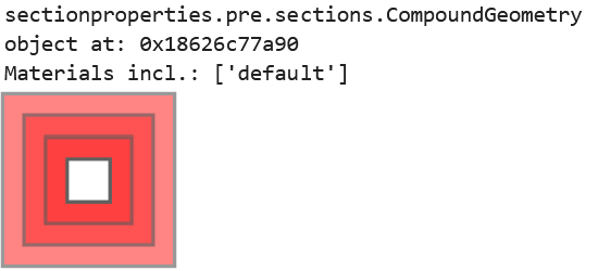
The nested geometry we are trying to create looks as follows:

In creating this geometry consider the following:

• shapely has a concept of “z-ordering” where it is possible for one geometry to be “over” another geometry and for an overlap section to exist. When a hole is created in a polygon, it is only local to that polygon.

• Triangle does not have a concept of “z-ordering” so there is only a single plane which may have regions of different materials (specified with control points). When a hole is created in the plane, it “punches” through “all” polygons in the plane.

To create the nested geometry using shapely, the code would be as follows:

mat1 = Material(name="Material 1", elastic_modulus=100, poissons_ratio=0.3, yield_strength=10, density=1e-6, color="yellow")
mat2 = Material(name="Material 2", elastic_modulus=100, poissons_ratio=0.3, yield_strength=10, density=1e-6, color="orange")
mat3 = Material(name="Material 3", elastic_modulus=100, poissons_ratio=0.3, yield_strength=10, density=1e-6, color="red")

sq1 = sections.rectangular_section(100, 100, material=mat1).align_center()
sq2 = sections.rectangular_section(75, 75, material=mat2).align_center()
sq3 = sections.rectangular_section(50, 50, material=mat3).align_center()
hole = sections.rectangular_section(25, 25).align_center()

compound = (
    (sq1 - sq2) # Create a big square with a medium hole in it and stack it over...
    + (sq2 - sq3) # ... a medium square with a medium-small hole in it and stack it over...
    + (sq3 - hole) # ...a medium-small square with a small hole in it.
)
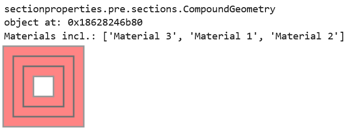
compound

To create the nested geometry using the Triangle interface, the code would be as follows:

points = [ # Points for four squares are created
    [-50.0, 50.0], # Square 1
    [50.0, 50.0],
    [50.0, -50.0],
    [-50.0, -50.0],
    [37.5, -37.5], # Square 2
    [37.5, 37.5],
    [-37.5, 37.5],
    [-37.5, -37.5],
    [25.0, -25.0], # Square 3
    [25.0, 25.0],
    [-25.0, 25.0],
    [-25.0, -25.0],
    [12.5, -12.5], # Square 4 (hole)
    [12.5, 12.5],
    [-12.5, 12.5],
    [-12.5, -12.5],
]

facets = [ # Facets trace each of the four squares
    [0, 1], # Square 1
    [1, 2],
    [2, 3],
    [3, 0],
    [4, 5], # Square 2
    [5, 6],
    [6, 7],
    [7, 4],
    [8, 9], # Square 3
    [9, 10],
    [10, 11],
    [11, 8],
    [12, 13], # Square 4 (hole)
    [13, 14],
    [14, 15],
    [15, 12],
]

control_points = [[-43.75, 0.0], [-31.25, 0.0], [-18.75, 0.0]] # Three squares
holes = [[0, 0]]

nested_compound = CompoundGeometry.from_points(
    points=points, facets=facets, control_points=control_points, holes=holes
)
nested_compound

Notice how the shapely representation shows the squares overlapping each other instead of the squares fitting into the “hole below”.

Is one of these methods better than the other? Not necessarily. The shapely approach is suitable for manually creating the geometry whereas the Triangle approach is suitable for reading in serialized data from a file, for example.

And, for either case, when the compound geometry is meshed, we see this: