Viewing the Results

Printing a List of the Section Properties

A list of section properties that have been calculated by various analyses can be printed to the terminal using the display_results() method that belongs to every Section object.

Section.display_results(fmt='8.6e')

Prints the results that have been calculated to the terminal.

Parameters

fmt (string) – Number formatting string

The following example displays the geometric section properties for a 100D x 50W rectangle with three digits after the decimal point:

import sectionproperties.pre.library.primitive_sections as primitive_sections
from sectionproperties.analysis.section import Section

geometry = primitive_sections.rectangular_section(d=100, b=50)
geometry.create_mesh(mesh_sizes=[5])

section = Section(geometry)
section.calculate_geometric_properties()

section.display_results(fmt='.3f')

Getting Specific Section Properties

Alternatively, there are a number of methods that can be called on the Section object to return a specific section property:

Section Area

Section.get_area()

Returns

Cross-section area

Return type

float

section = Section(geometry)
section.calculate_geometric_properties()
area = section.get_area()

Section Perimeter

Section.get_perimeter()

Returns

Cross-section perimeter

Return type

float

section = Section(geometry)
section.calculate_geometric_properties()
perimeter = section.get_perimeter()

Section Mass

Section.get_mass()

Returns

Cross-section mass

Return type

float

section = Section(geometry)
section.calculate_geometric_properties()
perimeter = section.get_mass()

Axial Rigidity

If material properties have been specified, returns the axial rigidity of the section.

Section.get_ea()

Returns

Modulus weighted area (axial rigidity)

Return type

float

section = Section(geometry)
section.calculate_geometric_properties()
ea = section.get_ea()

First Moments of Area

Section.get_q()

Returns

First moments of area about the global axis (qx, qy)

Return type

tuple(float, float)

section = Section(geometry)
section.calculate_geometric_properties()
(qx, qy) = section.get_q()

Second Moments of Area

Section.get_ig()

Returns

Second moments of area about the global axis (ixx_g, iyy_g, ixy_g)

Return type

tuple(float, float, float)

section = Section(geometry)
section.calculate_geometric_properties()
(ixx_g, iyy_g, ixy_g) = section.get_ig()

Section.get_ic()

Returns

Second moments of area centroidal axis (ixx_c, iyy_c, ixy_c)

Return type

tuple(float, float, float)

section = Section(geometry)
section.calculate_geometric_properties()
(ixx_c, iyy_c, ixy_c) = section.get_ic()

Section.get_ip()

Returns

Second moments of area about the principal axis (i11_c, i22_c)

Return type

tuple(float, float)

section = Section(geometry)
section.calculate_geometric_properties()
(i11_c, i22_c) = section.get_ip()

Elastic Centroid

Section.get_c()

Returns

Elastic centroid (cx, cy)

Return type

tuple(float, float)

section = Section(geometry)
section.calculate_geometric_properties()
(cx, cy) = section.get_c()

Section Moduli

Section.get_z()

Returns

Elastic section moduli about the centroidal axis with respect to the top and bottom fibres (zxx_plus, zxx_minus, zyy_plus, zyy_minus)

Return type

tuple(float, float, float, float)

section = Section(geometry)
section.calculate_geometric_properties()
(zxx_plus, zxx_minus, zyy_plus, zyy_minus) = section.get_z()

Section.get_zp()

Returns

Elastic section moduli about the principal axis with respect to the top and bottom fibres (z11_plus, z11_minus, z22_plus, z22_minus)

Return type

tuple(float, float, float, float)

section = Section(geometry)
section.calculate_geometric_properties()
(z11_plus, z11_minus, z22_plus, z22_minus) = section.get_zp()

Radii of Gyration

Section.get_rc()

Returns

Radii of gyration about the centroidal axis (rx, ry)

Return type

tuple(float, float)

section = Section(geometry)
section.calculate_geometric_properties()
(rx, ry) = section.get_rc()

Section.get_rp()

Returns

Radii of gyration about the principal axis (r11, r22)

Return type

tuple(float, float)

section = Section(geometry)
section.calculate_geometric_properties()
(r11, r22) = section.get_rp()

Principal Axis Angle

Section.get_phi()

Returns

Principal bending axis angle

Return type

float

section = Section(geometry)
section.calculate_geometric_properties()
phi = section.get_phi()

Effective Material Properties

Section.get_e_eff()

Returns

Effective elastic modulus based on area

Return type

float

section = Section(geometry)
section.calculate_warping_properties()
e_eff = section.get_e_eff()

Section.get_g_eff()

Returns

Effective shear modulus based on area

Return type

float

section = Section(geometry)
section.calculate_geometric_properties()
g_eff = section.get_g_eff()

Section.get_nu_eff()

Returns

Effective Poisson’s ratio

Return type

float

section = Section(geometry)
section.calculate_geometric_properties()
nu_eff = section.get_nu_eff()

Torsion Constant

Section.get_j()

Returns

St. Venant torsion constant

Return type

float

section = Section(geometry)
section.calculate_geometric_properties()
section.calculate_warping_properties()
j = section.get_j()

Shear Centre

Section.get_sc()

Returns

Centroidal axis shear centre (elasticity approach) (x_se, y_se)

Return type

tuple(float, float)

section = Section(geometry)
section.calculate_geometric_properties()
section.calculate_warping_properties()
(x_se, y_se) = section.get_sc()

Section.get_sc_p()

Returns

Principal axis shear centre (elasticity approach) (x11_se, y22_se)

Return type

tuple(float, float)

section = Section(geometry)
section.calculate_geometric_properties()
section.calculate_warping_properties()
(x11_se, y22_se) = section.get_sc_p()

Trefftz’s Shear Centre

Section.get_sc_t()

Returns

Centroidal axis shear centre (Trefftz’s approach) (x_st, y_st)

Return type

tuple(float, float)

section = Section(geometry)
section.calculate_geometric_properties()
section.calculate_warping_properties()
(x_st, y_st) = section.get_sc_t()

Warping Constant

Section.get_gamma()

Returns

Warping constant

Return type

float

section = Section(geometry)
section.calculate_geometric_properties()
section.calculate_warping_properties()
gamma = section.get_gamma()

Shear Area

Section.get_As()

Returns

Shear area for loading about the centroidal axis (A_sx, A_sy)

Return type

tuple(float, float)

section = Section(geometry)
section.calculate_geometric_properties()
section.calculate_warping_properties()
(A_sx, A_sy) = section.get_As()

Section.get_As_p()

Returns

Shear area for loading about the principal bending axis (A_s11, A_s22)

Return type

tuple(float, float)

section = Section(geometry)
section.calculate_geometric_properties()
section.calculate_warping_properties()
(A_s11, A_s22) = section.get_As_p()

Monosymmetry Constants

Section.get_beta()

Returns

Monosymmetry constant for bending about both global axes (beta_x_plus, beta_x_minus, beta_y_plus, beta_y_minus). The plus value relates to the top flange in compression and the minus value relates to the bottom flange in compression.

Return type

tuple(float, float, float, float)

section = Section(geometry)
section.calculate_geometric_properties()
section.calculate_warping_properties()
(beta_x_plus, beta_x_minus, beta_y_plus, beta_y_minus) = section.get_beta()

Section.get_beta_p()

Returns

Monosymmetry constant for bending about both principal axes (beta_11_plus, beta_11_minus, beta_22_plus, beta_22_minus). The plus value relates to the top flange in compression and the minus value relates to the bottom flange in compression.

Return type

tuple(float, float, float, float)

section = Section(geometry)
section.calculate_geometric_properties()
section.calculate_warping_properties()
(beta_11_plus, beta_11_minus, beta_22_plus, beta_22_minus) = section.get_beta_p()

Plastic Centroid

Section.get_pc()

Returns

Centroidal axis plastic centroid (x_pc, y_pc)

Return type

tuple(float, float)

section = Section(geometry)
section.calculate_geometric_properties()
section.calculate_plastic_properties()
(x_pc, y_pc) = section.get_pc()

Section.get_pc_p()

Returns

Principal bending axis plastic centroid (x11_pc, y22_pc)

Return type

tuple(float, float)

section = Section(geometry)
section.calculate_geometric_properties()
section.calculate_plastic_properties()
(x11_pc, y22_pc) = section.get_pc_p()

Plastic Section Moduli

Section.get_s()

Returns

Plastic section moduli about the centroidal axis (sxx, syy)

Return type

tuple(float, float)

If material properties have been specified, returns the plastic moment \(M_p = f_y S\).

section = Section(geometry)
section.calculate_geometric_properties()
section.calculate_plastic_properties()
(sxx, syy) = section.get_s()

Section.get_sp()

Returns

Plastic section moduli about the principal bending axis (s11, s22)

Return type

tuple(float, float)

If material properties have been specified, returns the plastic moment \(M_p = f_y S\).

section = Section(geometry)
section.calculate_geometric_properties()
section.calculate_plastic_properties()
(s11, s22) = section.get_sp()

Shape Factors

Section.get_sf()

Returns

Centroidal axis shape factors with respect to the top and bottom fibres (sf_xx_plus, sf_xx_minus, sf_yy_plus, sf_yy_minus)

Return type

tuple(float, float, float, float)

section = Section(geometry)
section.calculate_geometric_properties()
section.calculate_plastic_properties()
(sf_xx_plus, sf_xx_minus, sf_yy_plus, sf_yy_minus) = section.get_sf()

Section.get_sf_p()

Returns

Principal bending axis shape factors with respect to the top and bottom fibres (sf_11_plus, sf_11_minus, sf_22_plus, sf_22_minus)

Return type

tuple(float, float, float, float)

section = Section(geometry)
section.calculate_geometric_properties()
section.calculate_plastic_properties()
(sf_11_plus, sf_11_minus, sf_22_plus, sf_22_minus) = section.get_sf_p()

How Material Properties Affect Results

If a Geometry containing a user defined Material is used to build a Section, sectionproperties will assume you are performing a composite analysis and this will affect the way some of the results are stored and presented.

In general, the calculation of gross composite section properties takes into account the elastic modulus, Poisson’s ratio and yield strength of each material in the section. Unlike many design codes, sectionproperties is ‘material property agnostic’ and does not transform sections based on a defined material property, e.g. in reinforced concrete analysis it is commonplace to transform the reinforcing steel area based on the ratio between the elastic moduli, \(n = E_{steel} / E_{conc}\). sectionproperties instead calculates the gross material weighted properties, which is analogous to transforming with respect to a material property with elastic modulus, \(E = 1\).

Using the example of a reinforced concrete section, sectionproperties will calculate the gross section bending stiffness, \((EI)_g\), rather than an effective concrete second moment of area, \(I_{c,eff}\):

\[(EI)_g = E_s \times I_s + E_c \times I_c\]

If the user wanted to obtain the effective concrete second moment of area for a code calculation, they could simply divide the gross bending stiffness by the elastic modulus for concrete:

\[I_{c,eff} = \frac{(EI)_g}{E_c}\]

With reference to the get methods described in Printing a List of the Section Properties, a composite analysis will modify the following properties:

• First moments of area get_q() - returns elastic modulus weighted first moments of area \(E.Q\)

• Second moments of area get_ig(), get_ic(), get_ip() - return elastic modulus weighted second moments of area \(E.I\)

• Section moduli get_z(), get_zp() - return elastic modulus weighted section moduli \(E.Z\)

• Torsion constant get_j() - returns elastic modulus weighted torsion constant \(E.J\)

• Warping constant get_gamma() - returns elastic modulus weighted warping constant \(E.\Gamma\)

• Shear areas get_As(), get_As_p() - return elastic modulus weighted shear areas \(E.A_s\)

• Plastic section moduli get_s(), get_sp() - return yield strength weighted plastic section moduli, i.e. plastic moments \(M_p = f_y.S\)

A composite analysis will also enable the user to retrieve effective gross section area-weighted material properties:

• Effective elastic modulus \(E_{eff}\) - get_e_eff()

• Effective shear modulus \(G_{eff}\) - get_g_eff()

• Effective Poisson’s ratio \(\nu_{eff}\) - get_nu_eff()

These values may be used to transform composite properties output by sectionproperties for practical use, e.g. to calculate torsional rigidity:

\[(GJ)_g = \frac{G_{eff}}{E_{eff}} (EJ)_g\]

For further information, see the theoretical background to the calculation of Composite Cross-Sections.

Section Property Centroids Plots

A plot of the centroids (elastic, plastic and shear centre) can be produced with the finite element mesh in the background:

Section.plot_centroids(title='Centroids', **kwargs)

Plots the elastic centroid, the shear centre, the plastic centroids and the principal axis, if they have been calculated, on top of the finite element mesh.

Parameters

• title (string) – Plot title

• kwargs – Passed to plotting_context()

Returns

Matplotlib axes object

Return type

matplotlib.axes

The following example analyses a 200 PFC section and displays a plot of the centroids:

import sectionproperties.pre.library.steel_sections as steel_sections
from sectionproperties.analysis.section import Section

geometry = steel_sections.channel_section(d=200, b=75, t_f=12, t_w=6, r=12, n_r=8)
geometry.create_mesh(mesh_sizes=[20])

section = Section(geometry)
section.calculate_geometric_properties()
section.calculate_warping_properties()
section.calculate_plastic_properties()

section.plot_centroids()

Plot of the centroids generated by the above example.

The following example analyses a 150x90x12 UA section and displays a plot of the centroids:

import sectionproperties.pre.library.steel_sections as steel_sections
from sectionproperties.analysis.section import Section

geometry = steel_sections.angle_section(d=150, b=90, t=12, r_r=10, r_t=5, n_r=8)
geometry.create_mesh(mesh_sizes=[20])

section = Section(geometry)
section.calculate_geometric_properties()
section.calculate_warping_properties()
section.calculate_plastic_properties()

section.plot_centroids()

Plot of the centroids generated by the above example.

Plotting Section Stresses

There are a number of methods that can be called from a StressResult object to plot the various cross-section stresses. These methods take the following form:

StressResult.plot_(stress/vector)_(action)_(stresstype)

where:

• stress denotes a contour plot and vector denotes a vector plot.

• action denotes the type of action causing the stress e.g. mxx for bending moment about the x-axis. Note that the action is omitted for stresses caused by the application of all actions.

• stresstype denotes the type of stress that is being plotted e.g. zx for the x-component of shear stress.

The examples shown in the methods below are performed on a 150x90x12 UA (unequal angle) section. The Section object is created below:

import sectionproperties.pre.library.steel_sections as steel_sections
from sectionproperties.analysis.section import Section

geometry = steel_sections.AngleSection(d=150, b=90, t=12, r_r=10, r_t=5, n_r=8)
mesh = geometry.create_mesh(mesh_sizes=[2.5])
section = Section(geometry, mesh)

Primary Stress Plots

Axial Stress (\(\sigma_{zz,N}\))

StressPost.plot_stress_n_zz(title='Stress Contour Plot - $\\sigma_{zz,N}$', cmap='coolwarm', normalize=True, **kwargs)

Produces a contour plot of the normal stress \(\sigma_{zz,N}\) resulting from the axial load \(N\).

Parameters

• title (string) – Plot title

• cmap (string) – Matplotlib color map.

• normalize (bool) – If set to true, the CenteredNorm is used to scale the colormap. If set to false, the default linear scaling is used.

• kwargs – Passed to plotting_context()

Returns

Matplotlib axes object

Return type

matplotlib.axes

The following example plots the normal stress within a 150x90x12 UA section resulting from an axial force of 10 kN:

import sectionproperties.pre.library.steel_sections as steel_sections
from sectionproperties.analysis.section import Section

geometry = steel_sections.angle_section(d=150, b=90, t=12, r_r=10, r_t=5, n_r=8)
geometry.create_mesh(mesh_sizes=[20])
section = Section(geometry)

section.calculate_geometric_properties()
section.calculate_warping_properties()
stress_post = section.calculate_stress(N=10e3)

stress_post.plot_stress_n_zz()

Contour plot of the axial stress.

Bending Stress (\(\sigma_{zz,Mxx}\))

StressPost.plot_stress_mxx_zz(title='Stress Contour Plot - $\\sigma_{zz,Mxx}$', cmap='coolwarm', normalize=True, **kwargs)

Produces a contour plot of the normal stress \(\sigma_{zz,Mxx}\) resulting from the bending moment \(M_{xx}\).

Parameters

• title (string) – Plot title

• cmap (string) – Matplotlib color map.

• normalize (bool) – If set to true, the CenteredNorm is used to scale the colormap. If set to false, the default linear scaling is used.

• kwargs – Passed to plotting_context()

Returns

Matplotlib axes object

Return type

matplotlib.axes

The following example plots the normal stress within a 150x90x12 UA section resulting from a bending moment about the x-axis of 5 kN.m:

import sectionproperties.pre.library.steel_sections as steel_sections
from sectionproperties.analysis.section import Section

geometry = steel_sections.angle_section(d=150, b=90, t=12, r_r=10, r_t=5, n_r=8)
geometry.create_mesh(mesh_sizes=[20])
section = Section(geometry)

section.calculate_geometric_properties()
section.calculate_warping_properties()
stress_post = section.calculate_stress(Mxx=5e6)

stress_post.plot_stress_mxx_zz()

Contour plot of the bending stress.

Bending Stress (\(\sigma_{zz,Myy}\))

StressPost.plot_stress_myy_zz(title='Stress Contour Plot - $\\sigma_{zz,Myy}$', cmap='coolwarm', normalize=True, **kwargs)

Produces a contour plot of the normal stress \(\sigma_{zz,Myy}\) resulting from the bending moment \(M_{yy}\).

Parameters

• title (string) – Plot title

• cmap (string) – Matplotlib color map.

• normalize (bool) – If set to true, the CenteredNorm is used to scale the colormap. If set to false, the default linear scaling is used.

• kwargs – Passed to plotting_context()

Returns

Matplotlib axes object

Return type

matplotlib.axes

The following example plots the normal stress within a 150x90x12 UA section resulting from a bending moment about the y-axis of 2 kN.m:

import sectionproperties.pre.library.steel_sections as steel_sections
from sectionproperties.analysis.section import Section

geometry = steel_sections.angle_section(d=150, b=90, t=12, r_r=10, r_t=5, n_r=8)
geometry.create_mesh(mesh_sizes=[20])
section = Section(geometry)

section.calculate_geometric_properties()
section.calculate_warping_properties()
stress_post = section.calculate_stress(Myy=2e6)

stress_post.plot_stress_myy_zz()

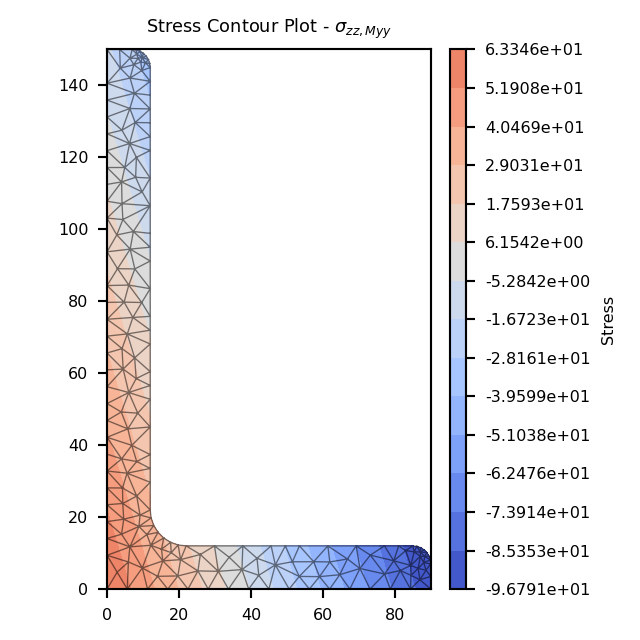
Contour plot of the bending stress.

Bending Stress (\(\sigma_{zz,M11}\))

StressPost.plot_stress_m11_zz(title='Stress Contour Plot - $\\sigma_{zz,M11}$', cmap='coolwarm', normalize=True, **kwargs)

Produces a contour plot of the normal stress \(\sigma_{zz,M11}\) resulting from the bending moment \(M_{11}\).

Parameters

• title (string) – Plot title

• cmap (string) – Matplotlib color map.

• normalize (bool) – If set to true, the CenteredNorm is used to scale the colormap. If set to false, the default linear scaling is used.

• kwargs – Passed to plotting_context()

Returns

Matplotlib axes object

Return type

matplotlib.axes

The following example plots the normal stress within a 150x90x12 UA section resulting from a bending moment about the 11-axis of 5 kN.m:

import sectionproperties.pre.library.steel_sections as steel_sections
from sectionproperties.analysis.section import Section

geometry = steel_sections.angle_section(d=150, b=90, t=12, r_r=10, r_t=5, n_r=8)
geometry.create_mesh(mesh_sizes=[20])
section = Section(geometry)

section.calculate_geometric_properties()
section.calculate_warping_properties()
stress_post = section.calculate_stress(M11=5e6)

stress_post.plot_stress_m11_zz()

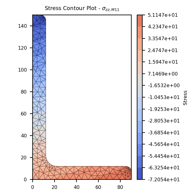
Contour plot of the bending stress.

Bending Stress (\(\sigma_{zz,M22}\))

StressPost.plot_stress_m22_zz(title='Stress Contour Plot - $\\sigma_{zz,M22}$', cmap='coolwarm', normalize=True, **kwargs)

Produces a contour plot of the normal stress \(\sigma_{zz,M22}\) resulting from the bending moment \(M_{22}\).

Parameters

• title (string) – Plot title

• cmap (string) – Matplotlib color map.

• normalize (bool) – If set to true, the CenteredNorm is used to scale the colormap. If set to false, the default linear scaling is used.

• kwargs – Passed to plotting_context()

Returns

Matplotlib axes object

Return type

matplotlib.axes

The following example plots the normal stress within a 150x90x12 UA section resulting from a bending moment about the 22-axis of 2 kN.m:

import sectionproperties.pre.library.steel_sections as steel_sections
from sectionproperties.analysis.section import Section

geometry = steel_sections.angle_section(d=150, b=90, t=12, r_r=10, r_t=5, n_r=8)
geometry.create_mesh(mesh_sizes=[20])
section = Section(geometry)

section.calculate_geometric_properties()
section.calculate_warping_properties()
stress_post = section.calculate_stress(M22=5e6)

stress_post.plot_stress_m22_zz()

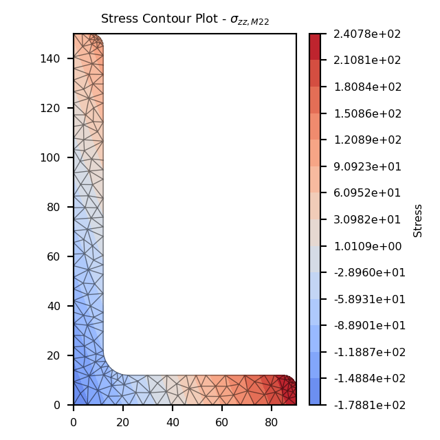
Contour plot of the bending stress.

Bending Stress (\(\sigma_{zz,\Sigma M}\))

StressPost.plot_stress_m_zz(title='Stress Contour Plot - $\\sigma_{zz,\\Sigma M}$', cmap='coolwarm', normalize=True, **kwargs)

Produces a contour plot of the normal stress \(\sigma_{zz,\Sigma M}\) resulting from all bending moments \(M_{xx} + M_{yy} + M_{11} + M_{22}\).

Parameters

• title (string) – Plot title

• cmap (string) – Matplotlib color map.

• normalize (bool) – If set to true, the CenteredNorm is used to scale the colormap. If set to false, the default linear scaling is used.

• kwargs – Passed to plotting_context()

Returns

Matplotlib axes object

Return type

matplotlib.axes

The following example plots the normal stress within a 150x90x12 UA section resulting from a bending moment about the x-axis of 5 kN.m, a bending moment about the y-axis of 2 kN.m and a bending moment of 3 kN.m about the 11-axis:

import sectionproperties.pre.library.steel_sections as steel_sections
from sectionproperties.analysis.section import Section

geometry = steel_sections.angle_section(d=150, b=90, t=12, r_r=10, r_t=5, n_r=8)
geometry.create_mesh(mesh_sizes=[20])
section = Section(geometry)

section.calculate_geometric_properties()
section.calculate_warping_properties()
stress_post = section.calculate_stress(Mxx=5e6, Myy=2e6, M11=3e6)

stress_post.plot_stress_m_zz()

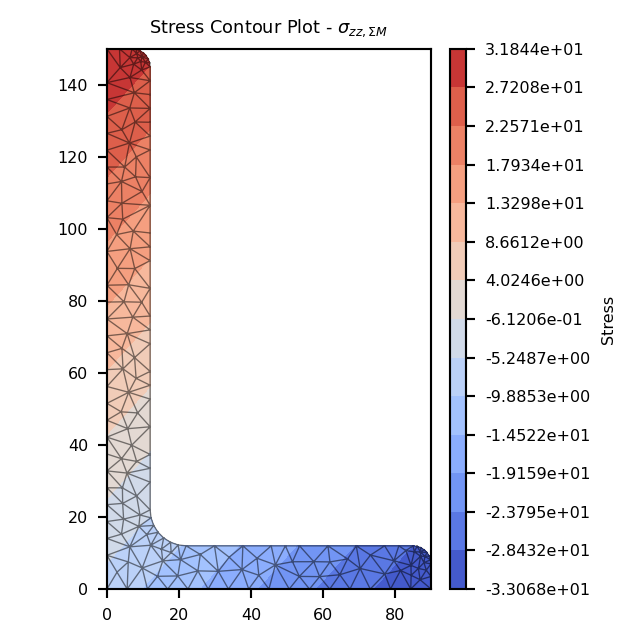
Contour plot of the bending stress.

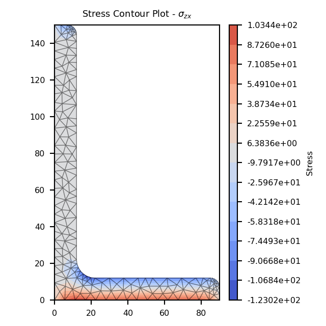
Torsion Stress (\(\sigma_{zx,Mzz}\))

StressPost.plot_stress_mzz_zx(title='Stress Contour Plot - $\\sigma_{zx,Mzz}$', cmap='coolwarm', normalize=True, **kwargs)

Produces a contour plot of the x-component of the shear stress \(\sigma_{zx,Mzz}\) resulting from the torsion moment \(M_{zz}\).

Parameters

• title (string) – Plot title

• cmap (string) – Matplotlib color map.

• normalize (bool) – If set to true, the CenteredNorm is used to scale the colormap. If set to false, the default linear scaling is used.

• kwargs – Passed to plotting_context()

Returns

Matplotlib axes object

Return type

matplotlib.axes

The following example plots the x-component of the shear stress within a 150x90x12 UA section resulting from a torsion moment of 1 kN.m:

import sectionproperties.pre.library.steel_sections as steel_sections
from sectionproperties.analysis.section import Section

geometry = steel_sections.angle_section(d=150, b=90, t=12, r_r=10, r_t=5, n_r=8)
geometry.create_mesh(mesh_sizes=[20])
section = Section(geometry)

section.calculate_geometric_properties()
section.calculate_warping_properties()
stress_post = section.calculate_stress(Mzz=1e6)

stress_post.plot_stress_mzz_zx()

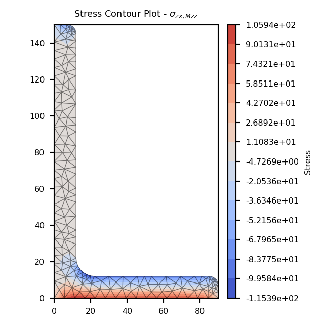
Contour plot of the shear stress.

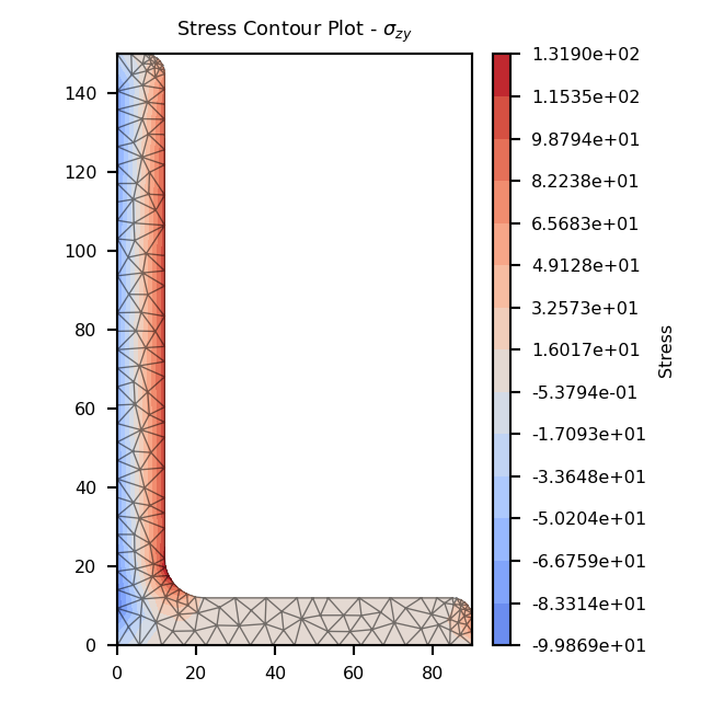
Torsion Stress (\(\sigma_{zy,Mzz}\))

StressPost.plot_stress_mzz_zy(title='Stress Contour Plot - $\\sigma_{zy,Mzz}$', cmap='coolwarm', normalize=True, **kwargs)

Produces a contour plot of the y-component of the shear stress \(\sigma_{zy,Mzz}\) resulting from the torsion moment \(M_{zz}\).

Parameters

• title (string) – Plot title

• cmap (string) – Matplotlib color map.

• normalize (bool) – If set to true, the CenteredNorm is used to scale the colormap. If set to false, the default linear scaling is used.

• kwargs – Passed to plotting_context()

Returns

Matplotlib axes object

Return type

matplotlib.axes

The following example plots the y-component of the shear stress within a 150x90x12 UA section resulting from a torsion moment of 1 kN.m:

import sectionproperties.pre.library.steel_sections as steel_sections
from sectionproperties.analysis.section import Section

geometry = steel_sections.angle_section(d=150, b=90, t=12, r_r=10, r_t=5, n_r=8)
geometry.create_mesh(mesh_sizes=[20])
section = Section(geometry)

section.calculate_geometric_properties()
section.calculate_warping_properties()
stress_post = section.calculate_stress(Mzz=1e6)

stress_post.plot_stress_mzz_zy()

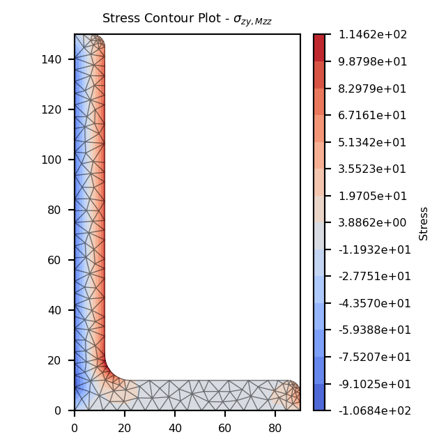
Contour plot of the shear stress.

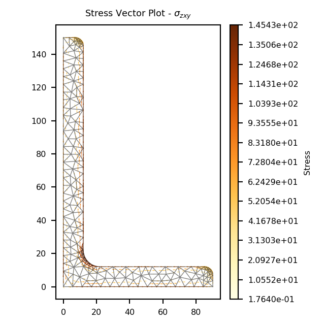
Torsion Stress (\(\sigma_{zxy,Mzz}\))

StressPost.plot_stress_mzz_zxy(title='Stress Contour Plot - $\\sigma_{zxy,Mzz}$', cmap='coolwarm', normalize=True, **kwargs)

Produces a contour plot of the resultant shear stress \(\sigma_{zxy,Mzz}\) resulting from the torsion moment \(M_{zz}\).

Parameters

• title (string) – Plot title

• cmap (string) – Matplotlib color map.

• normalize (bool) – If set to true, the CenteredNorm is used to scale the colormap. If set to false, the default linear scaling is used.

• kwargs – Passed to plotting_context()

Returns

Matplotlib axes object

Return type

matplotlib.axes

The following example plots a contour of the resultant shear stress within a 150x90x12 UA section resulting from a torsion moment of 1 kN.m:

import sectionproperties.pre.library.steel_sections as steel_sections
from sectionproperties.analysis.section import Section

geometry = steel_sections.angle_section(d=150, b=90, t=12, r_r=10, r_t=5, n_r=8)
geometry.create_mesh(mesh_sizes=[20])
section = Section(geometry)

section.calculate_geometric_properties()
section.calculate_warping_properties()
stress_post = section.calculate_stress(Mzz=1e6)

stress_post.plot_stress_mzz_zxy()

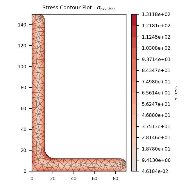
Contour plot of the shear stress.

StressPost.plot_vector_mzz_zxy(title='Stress Vector Plot - $\\sigma_{zxy,Mzz}$', cmap='YlOrBr', normalize=False, **kwargs)

Produces a vector plot of the resultant shear stress \(\sigma_{zxy,Mzz}\) resulting from the torsion moment \(M_{zz}\).

Parameters

• title (string) – Plot title

• cmap (string) – Matplotlib color map.

• normalize (bool) – If set to true, the CenteredNorm is used to scale the colormap. If set to false, the default linear scaling is used.

• kwargs – Passed to plotting_context()

Returns

Matplotlib axes object

Return type

matplotlib.axes

The following example generates a vector plot of the shear stress within a 150x90x12 UA section resulting from a torsion moment of 1 kN.m:

import sectionproperties.pre.library.steel_sections as steel_sections
from sectionproperties.analysis.section import Section

geometry = steel_sections.angle_section(d=150, b=90, t=12, r_r=10, r_t=5, n_r=8)
geometry.create_mesh(mesh_sizes=[20])
section = Section(geometry)

section.calculate_geometric_properties()
section.calculate_warping_properties()
stress_post = section.calculate_stress(Mzz=1e6)

stress_post.plot_vector_mzz_zxy()

Vector plot of the shear stress.

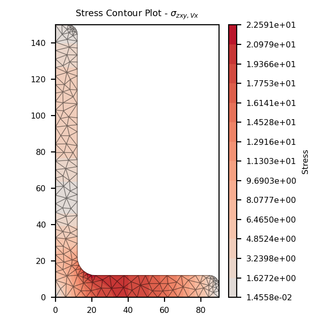
Shear Stress (\(\sigma_{zx,Vx}\))

StressPost.plot_stress_vx_zx(title='Stress Contour Plot - $\\sigma_{zx,Vx}$', cmap='coolwarm', normalize=True, **kwargs)

Produces a contour plot of the x-component of the shear stress \(\sigma_{zx,Vx}\) resulting from the shear force \(V_{x}\).

Parameters

• title (string) – Plot title

• cmap (string) – Matplotlib color map.

• normalize (bool) – If set to true, the CenteredNorm is used to scale the colormap. If set to false, the default linear scaling is used.

• kwargs – Passed to plotting_context()

Returns

Matplotlib axes object

Return type

matplotlib.axes

The following example plots the x-component of the shear stress within a 150x90x12 UA section resulting from a shear force in the x-direction of 15 kN:

import sectionproperties.pre.library.steel_sections as steel_sections
from sectionproperties.analysis.section import Section

geometry = steel_sections.angle_section(d=150, b=90, t=12, r_r=10, r_t=5, n_r=8)
geometry.create_mesh(mesh_sizes=[20])
section = Section(geometry)

section.calculate_geometric_properties()
section.calculate_warping_properties()
stress_post = section.calculate_stress(Vx=15e3)

stress_post.plot_stress_vx_zx()

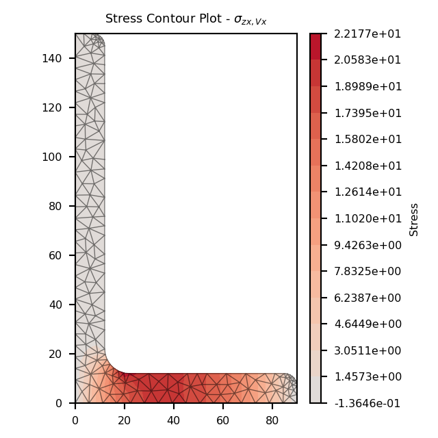
Contour plot of the shear stress.

Shear Stress (\(\sigma_{zy,Vx}\))

StressPost.plot_stress_vx_zy(title='Stress Contour Plot - $\\sigma_{zy,Vx}$', cmap='coolwarm', normalize=True, **kwargs)

Produces a contour plot of the y-component of the shear stress \(\sigma_{zy,Vx}\) resulting from the shear force \(V_{x}\).

Parameters

• title (string) – Plot title

• cmap (string) – Matplotlib color map.

• normalize (bool) – If set to true, the CenteredNorm is used to scale the colormap. If set to false, the default linear scaling is used.

• kwargs – Passed to plotting_context()

Returns

Matplotlib axes object

Return type

matplotlib.axes

The following example plots the y-component of the shear stress within a 150x90x12 UA section resulting from a shear force in the x-direction of 15 kN:

import sectionproperties.pre.library.steel_sections as steel_sections
from sectionproperties.analysis.section import Section

geometry = steel_sections.angle_section(d=150, b=90, t=12, r_r=10, r_t=5, n_r=8)
geometry.create_mesh(mesh_sizes=[20])
section = Section(geometry)

section.calculate_geometric_properties()
section.calculate_warping_properties()
stress_post = section.calculate_stress(Vx=15e3)

stress_post.plot_stress_vx_zy()

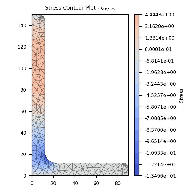
Contour plot of the shear stress.

Shear Stress (\(\sigma_{zxy,Vx}\))

StressPost.plot_stress_vx_zxy(title='Stress Contour Plot - $\\sigma_{zz,Myy}$', cmap='coolwarm', normalize=True, **kwargs)

Produces a contour plot of the resultant shear stress \(\sigma_{zxy,Vx}\) resulting from the shear force \(V_{x}\).

Parameters

• title (string) – Plot title

• cmap (string) – Matplotlib color map.

• normalize (bool) – If set to true, the CenteredNorm is used to scale the colormap. If set to false, the default linear scaling is used.

• kwargs – Passed to plotting_context()

Returns

Matplotlib axes object

Return type

matplotlib.axes

The following example plots a contour of the resultant shear stress within a 150x90x12 UA section resulting from a shear force in the x-direction of 15 kN:

import sectionproperties.pre.library.steel_sections as steel_sections
from sectionproperties.analysis.section import Section

geometry = steel_sections.angle_section(d=150, b=90, t=12, r_r=10, r_t=5, n_r=8)
geometry.create_mesh(mesh_sizes=[20])
section = Section(geometry)

section.calculate_geometric_properties()
section.calculate_warping_properties()
stress_post = section.calculate_stress(Vx=15e3)

stress_post.plot_stress_vx_zxy()

Contour plot of the shear stress.

StressPost.plot_vector_vx_zxy(title='Stress Vector Plot - $\\sigma_{zxy,Vx}$', cmap='YlOrBr', normalize=False, **kwargs)

Produces a vector plot of the resultant shear stress \(\sigma_{zxy,Vx}\) resulting from the shear force \(V_{x}\).

Parameters

• title (string) – Plot title

• cmap (string) – Matplotlib color map.

• normalize (bool) – If set to true, the CenteredNorm is used to scale the colormap. If set to false, the default linear scaling is used.

• kwargs – Passed to plotting_context()

Returns

Matplotlib axes object

Return type

matplotlib.axes

The following example generates a vector plot of the shear stress within a 150x90x12 UA section resulting from a shear force in the x-direction of 15 kN:

import sectionproperties.pre.library.steel_sections as steel_sections
from sectionproperties.analysis.section import Section

geometry = steel_sections.angle_section(d=150, b=90, t=12, r_r=10, r_t=5, n_r=8)
geometry.create_mesh(mesh_sizes=[20])
section = Section(geometry)

section.calculate_geometric_properties()
section.calculate_warping_properties()
stress_post = section.calculate_stress(Vx=15e3)

stress_post.plot_vector_vx_zxy()

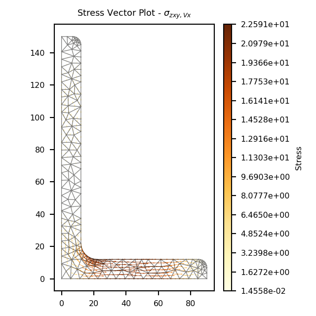
Vector plot of the shear stress.

Shear Stress (\(\sigma_{zx,Vy}\))

StressPost.plot_stress_vy_zx(title='Stress Contour Plot - $\\sigma_{zx,Vy}$', cmap='coolwarm', normalize=True, **kwargs)

Produces a contour plot of the x-component of the shear stress \(\sigma_{zx,Vy}\) resulting from the shear force \(V_{y}\).

Parameters

• title (string) – Plot title

• cmap (string) – Matplotlib color map.

• normalize (bool) – If set to true, the CenteredNorm is used to scale the colormap. If set to false, the default linear scaling is used.

• kwargs – Passed to plotting_context()

Returns

Matplotlib axes object

Return type

matplotlib.axes

The following example plots the x-component of the shear stress within a 150x90x12 UA section resulting from a shear force in the y-direction of 30 kN:

import sectionproperties.pre.library.steel_sections as steel_sections
from sectionproperties.analysis.section import Section

geometry = steel_sections.angle_section(d=150, b=90, t=12, r_r=10, r_t=5, n_r=8)
geometry.create_mesh(mesh_sizes=[20])
section = Section(geometry)

section.calculate_geometric_properties()
section.calculate_warping_properties()
stress_post = section.calculate_stress(Vy=30e3)

stress_post.plot_stress_vy_zx()

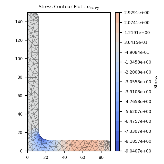
Contour plot of the shear stress.

Shear Stress (\(\sigma_{zy,Vy}\))

StressPost.plot_stress_vy_zy(title='Stress Contour Plot - $\\sigma_{zy,Vy}$', cmap='coolwarm', normalize=True, **kwargs)

Produces a contour plot of the y-component of the shear stress \(\sigma_{zy,Vy}\) resulting from the shear force \(V_{y}\).

Parameters

• title (string) – Plot title

• cmap (string) – Matplotlib color map.

• normalize (bool) – If set to true, the CenteredNorm is used to scale the colormap. If set to false, the default linear scaling is used.

• kwargs – Passed to plotting_context()

Returns

Matplotlib axes object

Return type

matplotlib.axes

The following example plots the y-component of the shear stress within a 150x90x12 UA section resulting from a shear force in the y-direction of 30 kN:

import sectionproperties.pre.library.steel_sections as steel_sections
from sectionproperties.analysis.section import Section

geometry = steel_sections.angle_section(d=150, b=90, t=12, r_r=10, r_t=5, n_r=8)
geometry.create_mesh(mesh_sizes=[20])
section = Section(geometry)

section.calculate_geometric_properties()
section.calculate_warping_properties()
stress_post = section.calculate_stress(Vy=30e3)

stress_post.plot_stress_vy_zy()

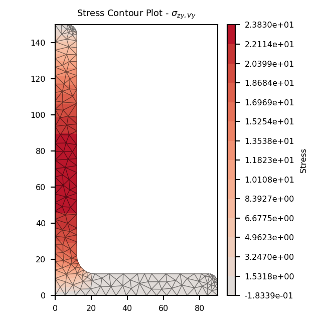
Contour plot of the shear stress.

Shear Stress (\(\sigma_{zxy,Vy}\))

StressPost.plot_stress_vy_zxy(title='Stress Contour Plot - $\\sigma_{zxy,Vy}$', cmap='coolwarm', normalize=True, **kwargs)

Produces a contour plot of the resultant shear stress \(\sigma_{zxy,Vy}\) resulting from the shear force \(V_{y}\).

Parameters

• title (string) – Plot title

• cmap (string) – Matplotlib color map.

• normalize (bool) – If set to true, the CenteredNorm is used to scale the colormap. If set to false, the default linear scaling is used.

• kwargs – Passed to plotting_context()

Returns

Matplotlib axes object

Return type

matplotlib.axes

The following example plots a contour of the resultant shear stress within a 150x90x12 UA section resulting from a shear force in the y-direction of 30 kN:

import sectionproperties.pre.library.steel_sections as steel_sections
from sectionproperties.analysis.section import Section

geometry = steel_sections.angle_section(d=150, b=90, t=12, r_r=10, r_t=5, n_r=8)
geometry.create_mesh(mesh_sizes=[20])
section = Section(geometry)

section.calculate_geometric_properties()
section.calculate_warping_properties()
stress_post = section.calculate_stress(Vy=30e3)

stress_post.plot_stress_vy_zxy()

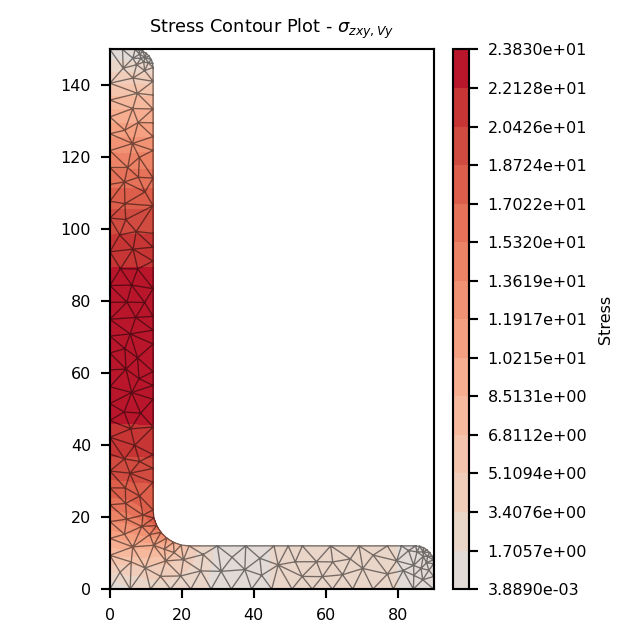
Contour plot of the shear stress.

StressPost.plot_vector_vy_zxy(title='Stress Vector Plot - $\\sigma_{zxy,Vy}$', cmap='YlOrBr', normalize=False, **kwargs)

Produces a vector plot of the resultant shear stress \(\sigma_{zxy,Vy}\) resulting from the shear force \(V_{y}\).

Parameters

• title (string) – Plot title

• cmap (string) – Matplotlib color map.

• normalize (bool) – If set to true, the CenteredNorm is used to scale the colormap. If set to false, the default linear scaling is used.

• kwargs – Passed to plotting_context()

Returns

Matplotlib axes object

Return type

matplotlib.axes

The following example generates a vector plot of the shear stress within a 150x90x12 UA section resulting from a shear force in the y-direction of 30 kN:

import sectionproperties.pre.library.steel_sections as steel_sections
from sectionproperties.analysis.section import Section

geometry = steel_sections.angle_section(d=150, b=90, t=12, r_r=10, r_t=5, n_r=8)
geometry.create_mesh(mesh_sizes=[20])
section = Section(geometry)

section.calculate_geometric_properties()
section.calculate_warping_properties()
stress_post = section.calculate_stress(Vy=30e3)

stress_post.plot_vector_vy_zxy()

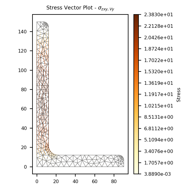
Vector plot of the shear stress.

Shear Stress (\(\sigma_{zx,\Sigma V}\))

StressPost.plot_stress_v_zx(title='Stress Contour Plot - $\\sigma_{zx,\\Sigma V}$', cmap='coolwarm', normalize=True, **kwargs)

Produces a contour plot of the x-component of the shear stress \(\sigma_{zx,\Sigma V}\) resulting from the sum of the applied shear forces \(V_{x} + V_{y}\).

Parameters

• title (string) – Plot title

• cmap (string) – Matplotlib color map.

• normalize (bool) – If set to true, the CenteredNorm is used to scale the colormap. If set to false, the default linear scaling is used.

• kwargs – Passed to plotting_context()

Returns

Matplotlib axes object

Return type

matplotlib.axes

The following example plots the x-component of the shear stress within a 150x90x12 UA section resulting from a shear force of 15 kN in the x-direction and 30 kN in the y-direction:

import sectionproperties.pre.library.steel_sections as steel_sections
from sectionproperties.analysis.section import Section

geometry = steel_sections.angle_section(d=150, b=90, t=12, r_r=10, r_t=5, n_r=8)
geometry.create_mesh(mesh_sizes=[20])
section = Section(geometry)

section.calculate_geometric_properties()
section.calculate_warping_properties()
stress_post = section.calculate_stress(Vx=15e3, Vy=30e3)

stress_post.plot_stress_v_zx()

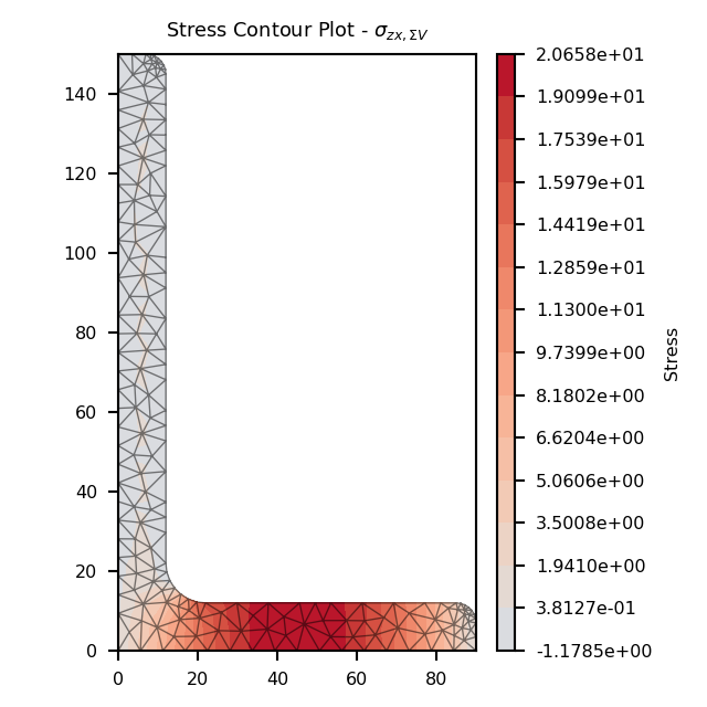
Contour plot of the shear stress.

Shear Stress (\(\sigma_{zy,\Sigma V}\))

StressPost.plot_stress_v_zy(title='Stress Contour Plot - $\\sigma_{zy,\\Sigma V}$', cmap='coolwarm', normalize=True, **kwargs)

Produces a contour plot of the y-component of the shear stress \(\sigma_{zy,\Sigma V}\) resulting from the sum of the applied shear forces \(V_{x} + V_{y}\).

Parameters

• title (string) – Plot title

• cmap (string) – Matplotlib color map.

• normalize (bool) – If set to true, the CenteredNorm is used to scale the colormap. If set to false, the default linear scaling is used.

• kwargs – Passed to plotting_context()

Returns

Matplotlib axes object

Return type

matplotlib.axes

The following example plots the y-component of the shear stress within a 150x90x12 UA section resulting from a shear force of 15 kN in the x-direction and 30 kN in the y-direction:

import sectionproperties.pre.library.steel_sections as steel_sections
from sectionproperties.analysis.section import Section

geometry = steel_sections.angle_section(d=150, b=90, t=12, r_r=10, r_t=5, n_r=8)
geometry.create_mesh(mesh_sizes=[20])
section = Section(geometry)

section.calculate_geometric_properties()
section.calculate_warping_properties()
stress_post = section.calculate_stress(Vx=15e3, Vy=30e3)

stress_post.plot_stress_v_zy()

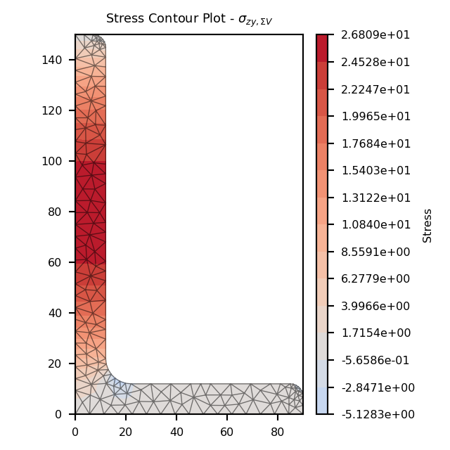
Contour plot of the shear stress.

Shear Stress (\(\sigma_{zxy,\Sigma V}\))

StressPost.plot_stress_v_zxy(title='Stress Contour Plot - $\\sigma_{zxy,\\Sigma V}$', cmap='coolwarm', normalize=True, **kwargs)

Produces a contour plot of the resultant shear stress \(\sigma_{zxy,\Sigma V}\) resulting from the sum of the applied shear forces \(V_{x} + V_{y}\).

Parameters

• title (string) – Plot title

• cmap (string) – Matplotlib color map.

• normalize (bool) – If set to true, the CenteredNorm is used to scale the colormap. If set to false, the default linear scaling is used.

• kwargs – Passed to plotting_context()

Returns

Matplotlib axes object

Return type

matplotlib.axes

The following example plots a contour of the resultant shear stress within a 150x90x12 UA section resulting from a shear force of 15 kN in the x-direction and 30 kN in the y-direction:

import sectionproperties.pre.library.steel_sections as steel_sections
from sectionproperties.analysis.section import Section

geometry = steel_sections.angle_section(d=150, b=90, t=12, r_r=10, r_t=5, n_r=8)
geometry.create_mesh(mesh_sizes=[20])
section = Section(geometry)

section.calculate_geometric_properties()
section.calculate_warping_properties()
stress_post = section.calculate_stress(Vx=15e3, Vy=30e3)

stress_post.plot_stress_v_zxy()

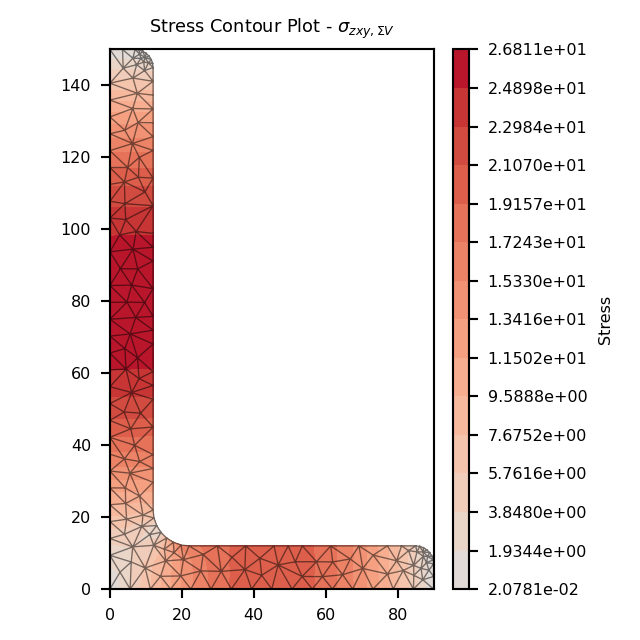
Contour plot of the shear stress.

StressPost.plot_vector_v_zxy(title='Stress Vector Plot - $\\sigma_{zxy,\\Sigma V}$', cmap='YlOrBr', normalize=False, **kwargs)

Produces a vector plot of the resultant shear stress \(\sigma_{zxy,\Sigma V}\) resulting from the sum of the applied shear forces \(V_{x} + V_{y}\).

Parameters

• title (string) – Plot title

• cmap (string) – Matplotlib color map.

• normalize (bool) – If set to true, the CenteredNorm is used to scale the colormap. If set to false, the default linear scaling is used.

• kwargs – Passed to plotting_context()

Returns

Matplotlib axes object

Return type

matplotlib.axes

The following example generates a vector plot of the shear stress within a 150x90x12 UA section resulting from a shear force of 15 kN in the x-direction and 30 kN in the y-direction:

import sectionproperties.pre.library.steel_sections as steel_sections
from sectionproperties.analysis.section import Section

geometry = steel_sections.angle_section(d=150, b=90, t=12, r_r=10, r_t=5, n_r=8)
geometry.create_mesh(mesh_sizes=[20])
section = Section(geometry)

section.calculate_geometric_properties()
section.calculate_warping_properties()
stress_post = section.calculate_stress(Vx=15e3, Vy=30e3)

stress_post.plot_vector_v_zxy()

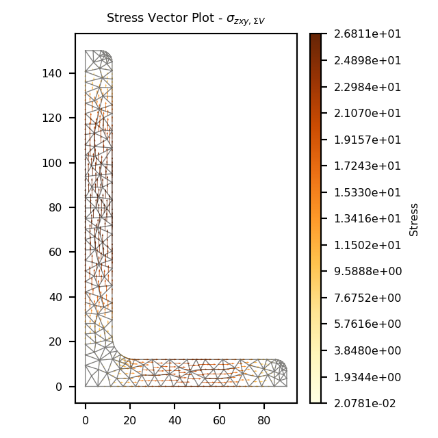
Vector plot of the shear stress.

Combined Stress Plots

Normal Stress (\(\sigma_{zz}\))

StressPost.plot_stress_zz(title='Stress Contour Plot - $\\sigma_{zz}$', cmap='coolwarm', normalize=True, **kwargs)

Produces a contour plot of the combined normal stress \(\sigma_{zz}\) resulting from all actions.

Parameters

• title (string) – Plot title

• cmap (string) – Matplotlib color map.

• normalize (bool) – If set to true, the CenteredNorm is used to scale the colormap. If set to false, the default linear scaling is used.

• kwargs – Passed to plotting_context()

Returns

Matplotlib axes object

Return type

matplotlib.axes

The following example plots the normal stress within a 150x90x12 UA section resulting from an axial force of 100 kN, a bending moment about the x-axis of 5 kN.m and a bending moment about the y-axis of 2 kN.m:

import sectionproperties.pre.library.steel_sections as steel_sections
from sectionproperties.analysis.section import Section

geometry = steel_sections.angle_section(d=150, b=90, t=12, r_r=10, r_t=5, n_r=8)
geometry.create_mesh(mesh_sizes=[20])
section = Section(geometry)

section.calculate_geometric_properties()
section.calculate_warping_properties()
stress_post = section.calculate_stress(N=100e3, Mxx=5e6, Myy=2e6)

stress_post.plot_stress_zz()

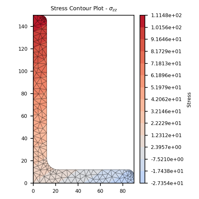
Contour plot of the normal stress.

Shear Stress (\(\sigma_{zx}\))

StressPost.plot_stress_zx(title='Stress Contour Plot - $\\sigma_{zx}$', cmap='coolwarm', normalize=True, **kwargs)

Produces a contour plot of the x-component of the shear stress \(\sigma_{zx}\) resulting from all actions.

Parameters

• title (string) – Plot title

• cmap (string) – Matplotlib color map.

• normalize (bool) – If set to true, the CenteredNorm is used to scale the colormap. If set to false, the default linear scaling is used.

• kwargs – Passed to plotting_context()

Returns

Matplotlib axes object

Return type

matplotlib.axes

The following example plots the x-component of the shear stress within a 150x90x12 UA section resulting from a torsion moment of 1 kN.m and a shear force of 30 kN in the y-direction:

import sectionproperties.pre.library.steel_sections as steel_sections
from sectionproperties.analysis.section import Section

geometry = steel_sections.angle_section(d=150, b=90, t=12, r_r=10, r_t=5, n_r=8)
geometry.create_mesh(mesh_sizes=[20])
section = Section(geometry)

section.calculate_geometric_properties()
section.calculate_warping_properties()
stress_post = section.calculate_stress(Mzz=1e6, Vy=30e3)

stress_post.plot_stress_zx()

Contour plot of the shear stress.

Shear Stress (\(\sigma_{zy}\))

StressPost.plot_stress_zy(title='Stress Contour Plot - $\\sigma_{zy}$', cmap='coolwarm', normalize=True, **kwargs)

Produces a contour plot of the y-component of the shear stress \(\sigma_{zy}\) resulting from all actions.

Parameters

• title (string) – Plot title

• cmap (string) – Matplotlib color map.

• normalize (bool) – If set to true, the CenteredNorm is used to scale the colormap. If set to false, the default linear scaling is used.

• kwargs – Passed to plotting_context()

Returns

Matplotlib axes object

Return type

matplotlib.axes

The following example plots the y-component of the shear stress within a 150x90x12 UA section resulting from a torsion moment of 1 kN.m and a shear force of 30 kN in the y-direction:

import sectionproperties.pre.library.steel_sections as steel_sections
from sectionproperties.analysis.section import Section

geometry = steel_sections.angle_section(d=150, b=90, t=12, r_r=10, r_t=5, n_r=8)
geometry.create_mesh(mesh_sizes=[20])
section = Section(geometry)

section.calculate_geometric_properties()
section.calculate_warping_properties()
stress_post = section.calculate_stress(Mzz=1e6, Vy=30e3)

stress_post.plot_stress_zy()

Contour plot of the shear stress.

Shear Stress (\(\sigma_{zxy}\))

StressPost.plot_stress_zxy(title='Stress Contour Plot - $\\sigma_{zxy}$', cmap='coolwarm', normalize=True, **kwargs)

Produces a contour plot of the resultant shear stress \(\sigma_{zxy}\) resulting from all actions.

Parameters

• title (string) – Plot title

• cmap (string) – Matplotlib color map.

• normalize (bool) – If set to true, the CenteredNorm is used to scale the colormap. If set to false, the default linear scaling is used.

• kwargs – Passed to plotting_context()

Returns

Matplotlib axes object

Return type

matplotlib.axes

The following example plots a contour of the resultant shear stress within a 150x90x12 UA section resulting from a torsion moment of 1 kN.m and a shear force of 30 kN in the y-direction:

import sectionproperties.pre.library.steel_sections as steel_sections
from sectionproperties.analysis.section import Section

geometry = steel_sections.angle_section(d=150, b=90, t=12, r_r=10, r_t=5, n_r=8)
geometry.create_mesh(mesh_sizes=[20])
section = Section(geometry)

section.calculate_geometric_properties()
section.calculate_warping_properties()
stress_post = section.calculate_stress(Mzz=1e6, Vy=30e3)

stress_post.plot_stress_zxy()

Contour plot of the shear stress.

StressPost.plot_vector_zxy(title='Stress Vector Plot - $\\sigma_{zxy}$', cmap='YlOrBr', normalize=False, **kwargs)

Produces a vector plot of the resultant shear stress \(\sigma_{zxy}\) resulting from all actions.

Parameters

• title (string) – Plot title

• cmap (string) – Matplotlib color map.

• normalize (bool) – If set to true, the CenteredNorm is used to scale the colormap. If set to false, the default linear scaling is used.

• kwargs – Passed to plotting_context()

Returns

Matplotlib axes object

Return type

matplotlib.axes

The following example generates a vector plot of the shear stress within a 150x90x12 UA section resulting from a torsion moment of 1 kN.m and a shear force of 30 kN in the y-direction:

import sectionproperties.pre.library.steel_sections as steel_sections
from sectionproperties.analysis.section import Section

geometry = steel_sections.angle_section(d=150, b=90, t=12, r_r=10, r_t=5, n_r=8)
geometry.create_mesh(mesh_sizes=[20])
section = Section(geometry)

section.calculate_geometric_properties()
section.calculate_warping_properties()
stress_post = section.calculate_stress(Mzz=1e6, Vy=30e3)

stress_post.plot_vector_zxy()

Vector plot of the shear stress.

Major Principal Stress (\(\sigma_{1}\))

StressPost.plot_stress_1(title='Stress Contour Plot - $\\sigma_{1}$', cmap='coolwarm', normalize=True, **kwargs)

Produces a contour plot of the major principal stress \(\sigma_{1}\) resulting from all actions.

Parameters

• title (string) – Plot title

• cmap (string) – Matplotlib color map.

• normalize (bool) – If set to true, the CenteredNorm is used to scale the colormap. If set to false, the default linear scaling is used.

• kwargs – Passed to plotting_context()

Returns

Matplotlib axes object

Return type

matplotlib.axes

The following example plots a contour of the major principal stress within a 150x90x12 UA section resulting from the following actions:

• \(N = 50\) kN

• \(M_{xx} = -5\) kN.m

• \(M_{22} = 2.5\) kN.m

• \(M_{zz} = 1.5\) kN.m

• \(V_{x} = 10\) kN

• \(V_{y} = 5\) kN

import sectionproperties.pre.library.steel_sections as steel_sections
from sectionproperties.analysis.section import Section

geometry = steel_sections.angle_section(d=150, b=90, t=12, r_r=10, r_t=5, n_r=8)
mesh = geometry.create_mesh(mesh_sizes=[2.5])
section = CrossSection(geometry, mesh)

section.calculate_geometric_properties()
section.calculate_warping_properties()
stress_post = section.calculate_stress(
    N=50e3, Mxx=-5e6, M22=2.5e6, Mzz=0.5e6, Vx=10e3, Vy=5e3
)

stress_post.plot_stress_1()

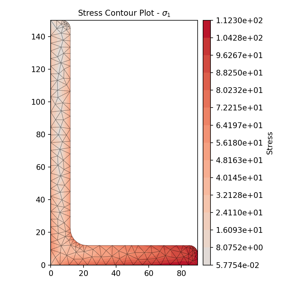
Contour plot of the major principal stress.

Minor Principal Stress (\(\sigma_{3}\))

StressPost.plot_stress_3(title='Stress Contour Plot - $\\sigma_{3}$', cmap='coolwarm', normalize=True, **kwargs)

Produces a contour plot of the Minor principal stress \(\sigma_{3}\) resulting from all actions.

Parameters

• title (string) – Plot title

• cmap (string) – Matplotlib color map.

• normalize (bool) – If set to true, the CenteredNorm is used to scale the colormap. If set to false, the default linear scaling is used.

• kwargs – Passed to plotting_context()

Returns

Matplotlib axes object

Return type

matplotlib.axes

The following example plots a contour of the Minor principal stress within a 150x90x12 UA section resulting from the following actions:

• \(N = 50\) kN

• \(M_{xx} = -5\) kN.m

• \(M_{22} = 2.5\) kN.m

• \(M_{zz} = 1.5\) kN.m

• \(V_{x} = 10\) kN

• \(V_{y} = 5\) kN

import sectionproperties.pre.library.steel_sections as steel_sections
from sectionproperties.analysis.section import Section

geometry = steel_sections.angle_section(d=150, b=90, t=12, r_r=10, r_t=5, n_r=8)
mesh = geometry.create_mesh(mesh_sizes=[2.5])
section = CrossSection(geometry, mesh)

section.calculate_geometric_properties()
section.calculate_warping_properties()
stress_post = section.calculate_stress(
    N=50e3, Mxx=-5e6, M22=2.5e6, Mzz=0.5e6, Vx=10e3, Vy=5e3
)

stress_post.plot_stress_3()

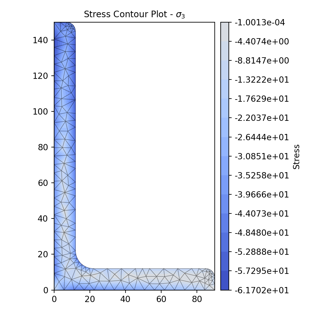
Contour plot of the minor principal stress.

von Mises Stress (\(\sigma_{vM}\))

StressPost.plot_stress_vm(title='Stress Contour Plot - $\\sigma_{vM}$', cmap='coolwarm', normalize=True, **kwargs)

Produces a contour plot of the von Mises stress \(\sigma_{vM}\) resulting from all actions.

Parameters

• title (string) – Plot title

• cmap (string) – Matplotlib color map.

• normalize (bool) – If set to true, the CenteredNorm is used to scale the colormap. If set to false, the default linear scaling is used.

• kwargs – Passed to plotting_context()

Returns

Matplotlib axes object

Return type

matplotlib.axes

The following example plots a contour of the von Mises stress within a 150x90x12 UA section resulting from the following actions:

• \(N = 50\) kN

• \(M_{xx} = -5\) kN.m

• \(M_{22} = 2.5\) kN.m

• \(M_{zz} = 1.5\) kN.m

• \(V_{x} = 10\) kN

• \(V_{y} = 5\) kN

import sectionproperties.pre.library.steel_sections as steel_sections
from sectionproperties.analysis.section import Section

geometry = steel_sections.angle_section(d=150, b=90, t=12, r_r=10, r_t=5, n_r=8)
geometry.create_mesh(mesh_sizes=[20])
section = Section(geometry)

section.calculate_geometric_properties()
section.calculate_warping_properties()
stress_post = section.calculate_stress(
    N=50e3, Mxx=-5e6, M22=2.5e6, Mzz=0.5e6, Vx=10e3, Vy=5e3
)

stress_post.plot_stress_vm()

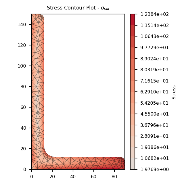
Contour plot of the von Mises stress.

Mohr’s Circles for Stresses at a Point

StressPost.plot_mohrs_circles(x, y, title=None, **kwargs)

Plots Mohr’s Circles of the 3D stress state at position x, y

Parameters

• x (float) – x-coordinate of the point to draw Mohr’s Circle

• y (float) – y-coordinate of the point to draw Mohr’s Circle

• title (string) – Plot title

• kwargs – Passed to plotting_context()

Returns

Matplotlib axes object

Return type

matplotlib.axes

The following example plots the Mohr’s Circles for the 3D stress state within a 150x90x12 UA section resulting from the following actions:

• \(N = 50\) kN

• \(M_{xx} = -5\) kN.m

• \(M_{22} = 2.5\) kN.m

• \(M_{zz} = 1.5\) kN.m

• \(V_{x} = 10\) kN

• \(V_{y} = 5\) kN

at the point (10, 88.9).

import sectionproperties.pre.library.steel_sections as steel_sections
from sectionproperties.analysis.section import Section

geometry = steel_sections.angle_section(d=150, b=90, t=12, r_r=10, r_t=5, n_r=8)
mesh = geometry.create_mesh(mesh_sizes=[2.5])
section = Section(geometry, mesh)

section.calculate_geometric_properties()
section.calculate_warping_properties()
stress_post = section.calculate_stress(
    N=50e3, Mxx=-5e6, M22=2.5e6, Mzz=0.5e6, Vx=10e3, Vy=5e3
)

stress_post.plot_mohrs_circles(10, 88.9)

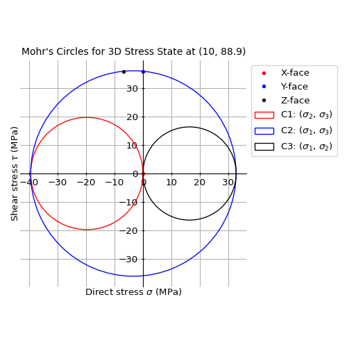
Mohr’s Circles of the 3D stress state at (10, 88.9).

Retrieving Section Stress

All cross-section stresses can be recovered using the get_stress() method that belongs to every StressPost object:

StressPost.get_stress()

Returns the stresses within each material belonging to the current StressPost object.

Returns

A list of dictionaries containing the cross-section stresses for each material.

Return type

list[dict]

A dictionary is returned for each material in the cross-section, containing the following keys and values:

• ‘Material’: Material name

• ‘sig_zz_n’: Normal stress \(\sigma_{zz,N}\) resulting from the axial load \(N\)

• ‘sig_zz_mxx’: Normal stress \(\sigma_{zz,Mxx}\) resulting from the bending moment \(M_{xx}\)

• ‘sig_zz_myy’: Normal stress \(\sigma_{zz,Myy}\) resulting from the bending moment \(M_{yy}\)

• ‘sig_zz_m11’: Normal stress \(\sigma_{zz,M11}\) resulting from the bending moment \(M_{11}\)

• ‘sig_zz_m22’: Normal stress \(\sigma_{zz,M22}\) resulting from the bending moment \(M_{22}\)

• ‘sig_zz_m’: Normal stress \(\sigma_{zz,\Sigma M}\) resulting from all bending moments

• ‘sig_zx_mzz’: x-component of the shear stress \(\sigma_{zx,Mzz}\) resulting from the torsion moment

• ‘sig_zy_mzz’: y-component of the shear stress \(\sigma_{zy,Mzz}\) resulting from the torsion moment

• ‘sig_zxy_mzz’: Resultant shear stress \(\sigma_{zxy,Mzz}\) resulting from the torsion moment

• ‘sig_zx_vx’: x-component of the shear stress \(\sigma_{zx,Vx}\) resulting from the shear force \(V_{x}\)

• ‘sig_zy_vx’: y-component of the shear stress \(\sigma_{zy,Vx}\) resulting from the shear force \(V_{x}\)

• ‘sig_zxy_vx’: Resultant shear stress \(\sigma_{zxy,Vx}\) resulting from the shear force \(V_{x}\)

• ‘sig_zx_vy’: x-component of the shear stress \(\sigma_{zx,Vy}\) resulting from the shear force \(V_{y}\)

• ‘sig_zy_vy’: y-component of the shear stress \(\sigma_{zy,Vy}\) resulting from the shear force \(V_{y}\)

• ‘sig_zxy_vy’: Resultant shear stress \(\sigma_{zxy,Vy}\) resulting from the shear force \(V_{y}\)

• ‘sig_zx_v’: x-component of the shear stress \(\sigma_{zx,\Sigma V}\) resulting from all shear forces

• ‘sig_zy_v’: y-component of the shear stress \(\sigma_{zy,\Sigma V}\) resulting from all shear forces

• ‘sig_zxy_v’: Resultant shear stress \(\sigma_{zxy,\Sigma V}\) resulting from all shear forces

• ‘sig_zz’: Combined normal stress \(\sigma_{zz}\) resulting from all actions

• ‘sig_zx’: x-component of the shear stress \(\sigma_{zx}\) resulting from all actions

• ‘sig_zy’: y-component of the shear stress \(\sigma_{zy}\) resulting from all actions

• ‘sig_zxy’: Resultant shear stress \(\sigma_{zxy}\) resulting from all actions

• ‘sig_1’: Major principal stress \(\sigma_{1}\) resulting from all actions

• ‘sig_3’: Minor principal stress \(\sigma_{3}\) resulting from all actions

• ‘sig_vm’: von Mises stress \(\sigma_{vM}\) resulting from all actions

The following example returns stresses for each material within a composite section, note that a result is generated for each node in the mesh for all materials irrespective of whether the materials exists at that point or not.

import sectionproperties.pre.library.steel_sections as steel_sections
from sectionproperties.analysis.section import Section

geometry = steel_sections.angle_section(d=150, b=90, t=12, r_r=10, r_t=5, n_r=8)
geometry.create_mesh(mesh_sizes=[20])
section = Section(geometry)

section.calculate_geometric_properties()
section.calculate_warping_properties()
stress_post = section.calculate_stress(
    N=50e3, Mxx=-5e6, M22=2.5e6, Mzz=0.5e6, Vx=10e3, Vy=5e3
)
stresses = stress_post.get_stress()

print("Number of nodes: {0}".format(section.num_nodes))

for stress in stresses:
    print('Material: {0}'.format(stress['Material']))
    print('List Size: {0}'.format(len(stress['sig_zz_n'])))
    print('Normal Stresses: {0}'.format(stress['sig_zz_n']))
    print('von Mises Stresses: {0}'.format(stress['sig_vm']))

$ Number of nodes: 2465

$ Material: Timber
$ List Size: 2465
$ Normal Stresses: [0.76923077 0.76923077 0.76923077 ... 0.76923077 0.76923077 0.76923077]
$ von Mises Stresses: [7.6394625  5.38571866 3.84784964 ... 3.09532948 3.66992556 2.81976647]

$ Material: Steel
$ List Size: 2465
$ Normal Stresses: [19.23076923 0. 0. ... 0. 0. 0.]
$ von Mises Stresses: [134.78886419 0. 0. ... 0. 0. 0.]