Composite Analysis
This example highlights how material properties allow composite analysis in sectionproperties.
Geometric vs. Composite
The default analysis type in sectionproperties is purely geometric, i.e. cross-section properties are reported based on the geometry only. In this analysis, all geometries are assigned the default material:
[1]:
from sectionproperties.analysis import Section
from sectionproperties.pre.library import rectangular_section

rect_geom = rectangular_section(d=100, b=50)
rect_geom.material
[1]:
Material(name='default', elastic_modulus=1, poissons_ratio=0, yield_strength=1, density=1, color='w')
The default material has a unit elastic modulus, yield strength and density, and a Poisson’s ratio of zero.
Geometric-only analysis allows geometric properties to be obtained:
[2]:
rect_geom.create_mesh(mesh_sizes=10)  # create mesh
rect_sec = Section(geometry=rect_geom)
rect_sec.calculate_geometric_properties()
ixx, iyy, ixy = rect_sec.get_ic()  # get second moments of area
print(f"Ixx = {ixx:.5e} mm4")
Ixx = 4.16667e+06 mm4
When a material property gets added to a geometry, the analysis becomes composite.
[3]:
from sectionproperties.pre import Material

# assign steel to the geometry
steel = Material(
    name="Steel",
    elastic_modulus=200e3,
    poissons_ratio=0.3,
    density=7.85e-6,
    yield_strength=500,
    color="grey",
)
rect_geom.material = steel

# recreate mesh and section
rect_geom.create_mesh(mesh_sizes=10)
rect_sec = Section(geometry=rect_geom)
rect_sec.calculate_geometric_properties()
Cross-section properties are now modulus weighted as the assumption is that there are multiple regions with multiple different material properties. We can no longer obtain geometric-only properties:
[4]:
ixx, iyy, ixy = rect_sec.get_ic() # get second moments of area
---------------------------------------------------------------------------
RuntimeError                              Traceback (most recent call last)
Cell In[4], line 1
----> 1 ixx, iyy, ixy = rect_sec.get_ic()  # get second moments of area

File ~/checkouts/readthedocs.org/user_builds/sectionproperties/checkouts/stable/src/sectionproperties/analysis/section.py:2203, in Section.get_ic(self)
   2201     msg = "Attempting to get a geometric only property for a composite analysis"
   2202     msg += " (material properties have been applied). Consider using get_eic()."
-> 2203     raise RuntimeError(msg)
   2205 if (
   2206     self.section_props.ixx_c is None
   2207     or self.section_props.ixy_c is None
   2208     or self.section_props.iyy_c is None
   2209 ):
   2210     msg = "Conduct a geometric analysis."

RuntimeError: Attempting to get a geometric only property for a composite analysis (material properties have been applied). Consider using get_eic().
In this case, we need to get the modulus weighted second moments of area. Note we can still extract geometric properties by using a reference elastic modulus.
[5]:
# get modulus weighted second moments of area
eixx, eiyy, eixy = rect_sec.get_eic()
print(f"E.Ixx = {eixx:.5e} N.mm2")

# use reference elastic modulus to get transformed properties
ixx, iyy, ixy = rect_sec.get_eic(e_ref=steel)
print(f"Ixx = {ixx:.5e} mm4")
E.Ixx = 8.33333e+11 N.mm2
Ixx = 4.16667e+06 mm4
Steel-Timber Composite Section
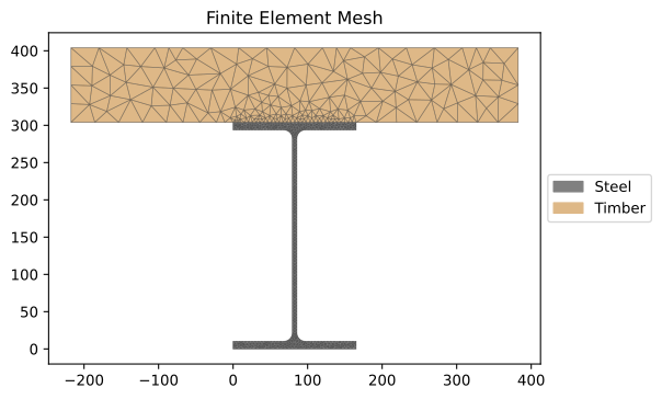
The following section models a composite timber floor and steel beam section. A universal steel beam (310UB40.4) is modelled with a 100D x 600W timber panel placed on its top flange.
Create the Materials
[6]:
# create the steel material
steel = Material(
    name="Steel",
    elastic_modulus=200e3,
    poissons_ratio=0.3,
    density=7.85e-6,
    yield_strength=500,
    color="grey",
)

# create the timber material
timber = Material(
    name="Timber",
    elastic_modulus=8e3,
    poissons_ratio=0.35,
    yield_strength=20,
    density=0.78e-6,
    color="burlywood",
)
Create the Geometry
[7]:
from sectionproperties.pre.library import i_section

# universal steel beam
ub = i_section(d=304, b=165, t_f=10.2, t_w=6.1, r=11.4, n_r=8, material=steel)

# timber floor panel
panel = rectangular_section(d=100, b=600, material=timber)
panel = panel.align_center(align_to=ub).align_to(other=ub, on="top")

# combine geometry
geom = ub + panel
Create Mesh and Section Object
[8]:
# 10 mm2 mesh for UB, 500 mm2 mesh for timber
geom.create_mesh(mesh_sizes=[10, 500])
sec = Section(geometry=geom)
sec.plot_mesh()
[8]:
<Axes: title={'center': 'Finite Element Mesh'}>
Perform Analysis
[9]:
sec.calculate_geometric_properties()
sec.calculate_warping_properties()
sec.calculate_plastic_properties()
Display Analysis Results
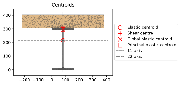
We can plot the various centroids found by the analyses.
[10]:
sec.plot_centroids()
[10]:
<Axes: title={'center': 'Centroids'}>
We can also print all the calculated section properties to the terminal, note that because have conducted a composite analysis, modulus weighted properties are displayed.
[11]:
sec.display_results()
     Section Properties
┏━━━━━━━━━━━┳━━━━━━━━━━━━━━━┓
┃ Property  ┃         Value ┃
┡━━━━━━━━━━━╇━━━━━━━━━━━━━━━┩
│ area      │  6.521094e+04 │
│ perimeter │  2.306078e+03 │
│ mass      │  8.770585e-02 │
│ e.a       │  1.522187e+09 │
│ e.qx      │  3.283325e+11 │
│ e.qy      │  1.255805e+11 │
│ e.ixx_g   │  1.019283e+14 │
│ e.iyy_g   │  2.628963e+13 │
│ e.ixy_g   │  2.708743e+13 │
│ cx        │  8.250000e+01 │
│ cy        │  2.156978e+02 │
│ e.ixx_c   │  3.110771e+13 │
│ e.iyy_c   │  1.592924e+13 │
│ e.ixy_c   │ -9.375000e-02 │
│ e.zxx+    │  1.652010e+11 │
│ e.zxx-    │  1.442190e+11 │
│ e.zyy+    │  5.309747e+10 │
│ e.zyy-    │  5.309747e+10 │
│ my_xx     │  3.605474e+08 │
│ my_yy     │  1.327437e+08 │
│ rx        │  1.429552e+02 │
│ ry        │  1.022971e+02 │
│ e.i11_c   │  3.110771e+13 │
│ e.i22_c   │  1.592924e+13 │
│ phi       │  0.000000e+00 │
│ e.z11+    │  1.652010e+11 │
│ e.z11-    │  1.442190e+11 │
│ e.z22+    │  5.309747e+10 │
│ e.z22-    │  5.309747e+10 │
│ my_11     │  3.605474e+08 │
│ my_22     │  1.327437e+08 │
│ r11       │  1.429552e+02 │
│ r22       │  1.022971e+02 │
│ e_eff     │  2.334252e+04 │
│ g_eff     │  8.873037e+03 │
│ nu_eff    │  3.153622e-01 │
│ e.j       │  2.169153e+12 │
│ x_se      │  8.255462e+01 │
│ y_se      │  3.200131e+02 │
│ x1_se     │  5.461533e-02 │
│ y2_se     │  1.043152e+02 │
│ x_st      │  8.255367e+01 │
│ y_st      │  3.179106e+02 │
│ e.gamma   │  8.613474e+16 │
│ e.a_sx    │  6.005132e+08 │
│ e.a_sy    │  4.252562e+08 │
│ e.a_s11   │  6.005132e+08 │
│ e.a_s22   │  4.252562e+08 │
│ beta_x+   │  2.165060e+02 │
│ beta_x-   │ -2.165060e+02 │
│ beta_y+   │  1.092307e-01 │
│ beta_y-   │ -1.092307e-01 │
│ beta_11+  │  2.165060e+02 │
│ beta_11-  │ -2.165060e+02 │
│ beta_22+  │  1.092307e-01 │
│ beta_22-  │ -1.092307e-01 │
│ x_pc      │  8.250000e+01 │
│ y_pc      │  2.954820e+02 │
│ x11_pc    │  8.250000e+01 │
│ y22_pc    │  2.954820e+02 │
│ mp_xx     │  4.500453e+08 │
│ mp_yy     │  2.510673e+08 │
│ mp_11     │  4.500453e+08 │
│ mp_22     │  2.510673e+08 │
│ sf_xx+    │  1.248228e+00 │
│ sf_xx-    │  1.248228e+00 │
│ sf_yy+    │  1.891369e+00 │
│ sf_yy-    │  1.891369e+00 │
│ sf_11+    │  1.248228e+00 │
│ sf_11-    │  1.248228e+00 │
│ sf_22+    │  1.891369e+00 │
│ sf_22-    │  1.891369e+00 │
└───────────┴───────────────┘
We can also get transformed properties by specifying a reference material.
[12]:
ixx_timber, _, _ = sec.get_eic(e_ref=timber)
ixx_steel, _, _ = sec.get_eic(e_ref=steel)
print(f"Ixx,t = {ixx_timber:.3e} mm4")
print(f"Ixx,s = {ixx_steel:.3e} mm4")
Ixx,t = 3.888e+09 mm4
Ixx,s = 1.555e+08 mm4
Further, we can display the transformed results with respect to an elastic modulus by calling the display_transformed_results() method. Here we print the transformed section properties with respect to the timber.
[13]:
sec.display_transformed_results(e_ref=timber)
     Transformed Section
         Properties
┏━━━━━━━━━━━┳━━━━━━━━━━━━━━━┓
┃ Property  ┃         Value ┃
┡━━━━━━━━━━━╇━━━━━━━━━━━━━━━┩
│ geom area │  6.521094e+04 │
│ perimeter │  2.306078e+03 │
│ mass      │  8.770585e-02 │
│ e_ref     │  8.000000e+03 │
│ a         │  1.902734e+05 │
│ qx        │  4.104156e+07 │
│ qy        │  1.569756e+07 │
│ ixx_g     │  1.274104e+10 │
│ iyy_g     │  3.286203e+09 │
│ ixy_g     │  3.385929e+09 │
│ cx        │  8.250000e+01 │
│ cy        │  2.156978e+02 │
│ ixx_c     │  3.888464e+09 │
│ iyy_c     │  1.991155e+09 │
│ ixy_c     │ -1.171875e-05 │
│ zxx+      │  2.065013e+07 │
│ zxx-      │  1.802737e+07 │
│ zyy+      │  6.637183e+06 │
│ zyy-      │  6.637183e+06 │
│ my_xx     │  3.605474e+08 │
│ my_yy     │  1.327437e+08 │
│ rx        │  1.429552e+02 │
│ ry        │  1.022971e+02 │
│ i11_c     │  3.888464e+09 │
│ i22_c     │  1.991155e+09 │
│ phi       │  0.000000e+00 │
│ z11+      │  2.065013e+07 │
│ z11-      │  1.802737e+07 │
│ z22+      │  6.637183e+06 │
│ z22-      │  6.637183e+06 │
│ my_11     │  3.605474e+08 │
│ my_22     │  1.327437e+08 │
│ r11       │  1.429552e+02 │
│ r22       │  1.022971e+02 │
│ e_eff     │  2.334252e+04 │
│ g_eff     │  8.873037e+03 │
│ nu_eff    │  3.153622e-01 │
│ j         │  2.711441e+08 │
│ x_se      │  8.255462e+01 │
│ y_se      │  3.200131e+02 │
│ x1_se     │  5.461533e-02 │
│ y2_se     │  1.043152e+02 │
│ x_st      │  8.255367e+01 │
│ y_st      │  3.179106e+02 │
│ gamma     │  1.076684e+13 │
│ a_sx      │  7.506415e+04 │
│ a_sy      │  5.315702e+04 │
│ a_s11     │  7.506415e+04 │
│ a_s22     │  5.315702e+04 │
│ beta_x+   │  2.165060e+02 │
│ beta_x-   │ -2.165060e+02 │
│ beta_y+   │  1.092307e-01 │
│ beta_y-   │ -1.092307e-01 │
│ beta_11+  │  2.165060e+02 │
│ beta_11-  │ -2.165060e+02 │
│ beta_22+  │  1.092307e-01 │
│ beta_22-  │ -1.092307e-01 │
│ x_pc      │  8.250000e+01 │
│ y_pc      │  2.954820e+02 │
│ x11_pc    │  8.250000e+01 │
│ y22_pc    │  2.954820e+02 │
│ mp_xx     │  4.500453e+08 │
│ mp_yy     │  2.510673e+08 │
│ mp_11     │  4.500453e+08 │
│ mp_22     │  2.510673e+08 │
│ sf_xx+    │  1.248228e+00 │
│ sf_xx-    │  1.248228e+00 │
│ sf_yy+    │  1.891369e+00 │
│ sf_yy-    │  1.891369e+00 │
│ sf_11+    │  1.248228e+00 │
│ sf_11-    │  1.248228e+00 │
│ sf_22+    │  1.891369e+00 │
│ sf_22-    │  1.891369e+00 │
└───────────┴───────────────┘
A plastic analysis for composite sections will calculate plastic moments rather than plastic section moduli. The plastic moment assumes all geometry fibres reach the yield strength.
[14]:
mp_xx, _ = sec.get_mp()
print(f"Mp = {mp_xx / 1e6:.1f} kN.m")
Mp = 450.0 kN.m
Stress Analysis
[15]:
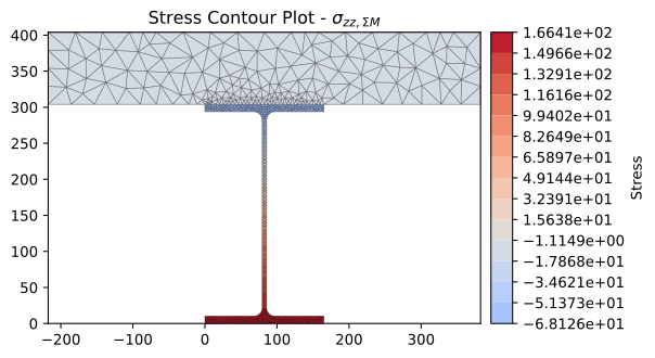
stress = sec.calculate_stress(n=-100e3, mxx=-120e6, vy=-75e3)
[16]:
stress.plot_stress(stress="m_zz")
[16]:
<Axes: title={'center': 'Stress Contour Plot - $\\sigma_{zz,\\Sigma M}$'}>
[17]:
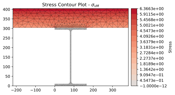
stress.plot_stress(stress="vm")
[17]:
<Axes: title={'center': 'Stress Contour Plot - $\\sigma_{vM}$'}>
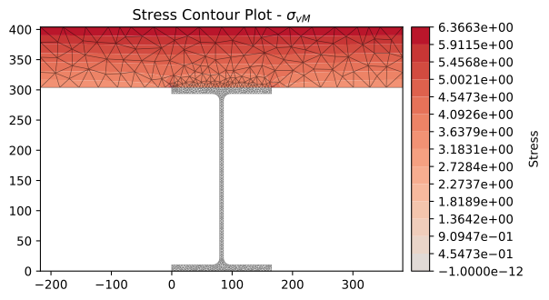
We can plot only a specific list of materials by including the material_list argument. In the above plot it is difficult to see the stress in the timber so we set material_list=[timber].
[18]:
stress.plot_stress(stress="vm", material_list=[timber])
[18]:
<Axes: title={'center': 'Stress Contour Plot - $\\sigma_{vM}$'}>